5 Validate using reduced sampling data
In chapter 2 we found the optimal power settings for the Tydal and Geilo sites. Now I just want to look at how this might have changed when we have removed superflous data points as in chapter 3.
Lets say for Tydal that we want to have 20 meters between the sampling points.
tm_shape(SHP_tydal) + tm_polygons() + tm_shape(depths_tydal_i60) +
    tm_dots(size = "Dybde", scale = 2, col = "Dybde",
        palette = "-viridis", title = "Measured peat depth (m)") +
    tm_layout(legend.outside = T)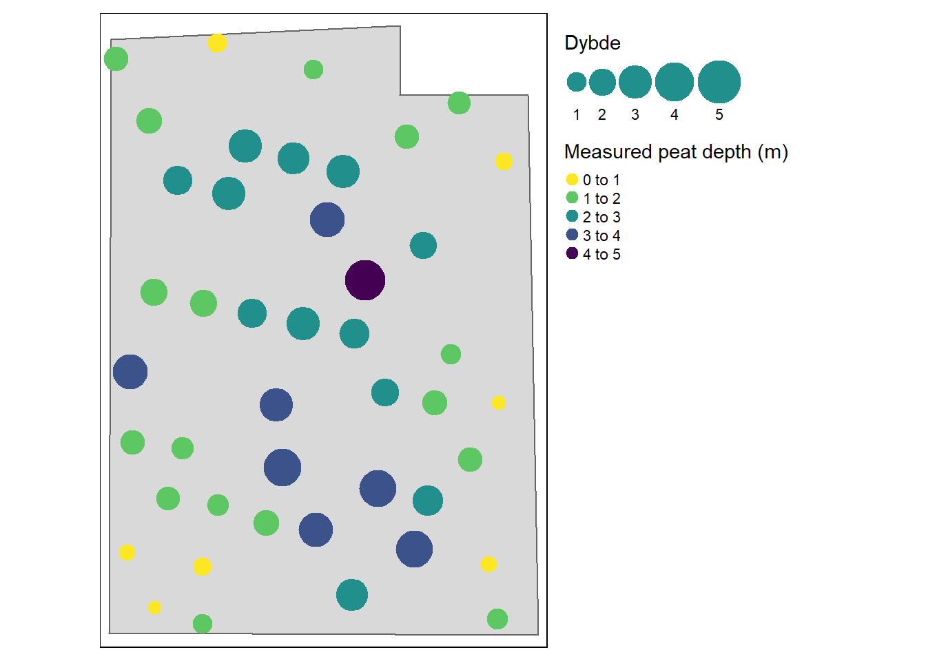
Figure 5.1: Peat depth measurements in the Tydal test site, after trimming the data poins so that the median distance between them is 20 meters.
Confirm the median distance is 20 meters
temp <- sf::st_distance(depths_tydal_i60)
temp <- units::drop_units(temp)
temp[temp == 0] <- NA
temp <- rowMins(temp, na.rm = T)
median(temp)
#> [1] 20.18216
Then we determine the optimal power setting.
ccalc_optimumPower <- function(powerRange = 1:6, nmax = 20,
    peatDepths, peatlandDelimination, title) {

    temp <- data.frame(power = powerRange, MAE = as.numeric(NA))

    vol <- NULL

    myGrid <- starsExtra::make_grid(peatlandDelimination,
        1)
    myGrid <- sf::st_crop(myGrid, peatlandDelimination)

    for (i in powerRange) {

        # Get the MAE
        temp2 <- krige.cv(Dybde ~ 1, peatDepths, set = list(idp = i),
            nmax = nmax)
        temp$MAE[temp$power == i] <- mean(abs(temp2$residual))

        # Get the volume
        vol_temp <- gstat::idw(Dybde ~ 1, peatDepths,
            newdata = myGrid, nmax = nmax, idp = i)

        vol <- c(vol, sum(vol_temp$var1.pred, na.rm = T))
    }

    ifelse(temp$power[which.min(temp$MAE)] < 2, temp$best <- ifelse(temp$power ==
        2, "best", "not-best"), temp$best <- ifelse(temp$MAE ==
        min(temp$MAE), "best", "not-best"))

    # Plot MAE
    gg_out <- ggplot(temp, aes(x = power, y = MAE,
        colour = best, shape = best)) + geom_point(size = 10) +
        theme_bw(base_size = 12) + scale_x_continuous(breaks = powerRange) +
        guides(colour = "none", shape = "none") + scale_color_manual(values = c("darkgreen",
        "grey")) + scale_shape_manual(values = c(18,
        19)) + ggtitle(title)

    # Plot volume
    vol_df <- data.frame(volume = vol, power = powerRange)
    vol_df$relative_volume <- vol_df$volume/mean(vol_df$volume) *
        100

    gg_out_vol <- ggplot(vol_df, aes(x = factor(power),
        y = relative_volume)) + geom_point(size = 8) +
        xlab("power") + ylab("Peat volume as a percentage of\nmean predicted peat volume") +
        theme_bw(base_size = 12)

    ggpubr::ggarrange(gg_out, gg_out_vol)
}ccalc_optimumPower(peatDepths = depths_tydal_i60, title = "Tydal",
peatlandDelimination = SHP_tydal)
#>
|
| | 0%
|
|= | 2%
|
|== | 5%
|
|=== | 7%
|
|===== | 9%
|
|====== | 12%
|
|======= | 14%
|
|======== | 16%
|
|========= | 19%
|
|========== | 21%
|
|============ | 23%
|
|============= | 26%
|
|============== | 28%
|
|=============== | 30%
|
|================ | 33%
|
|================= | 35%
|
|=================== | 37%
|
|==================== | 40%
|
|===================== | 42%
|
|====================== | 44%
|
|======================= | 47%
|
|======================== | 49%
|
|========================== | 51%
|
|=========================== | 53%
|
|============================ | 56%
|
|============================= | 58%
|
|============================== | 60%
|
|=============================== | 63%
|
|================================= | 65%
|
|================================== | 67%
|
|=================================== | 70%
|
|==================================== | 72%
|
|===================================== | 74%
|
|====================================== | 77%
|
|======================================== | 79%
|
|========================================= | 81%
|
|========================================== | 84%
|
|=========================================== | 86%
|
|============================================ | 88%
|
|============================================= | 91%
|
|=============================================== | 93%
|
|================================================ | 95%
|
|================================================= | 98%
|
|==================================================| 100%
#> [inverse distance weighted interpolation]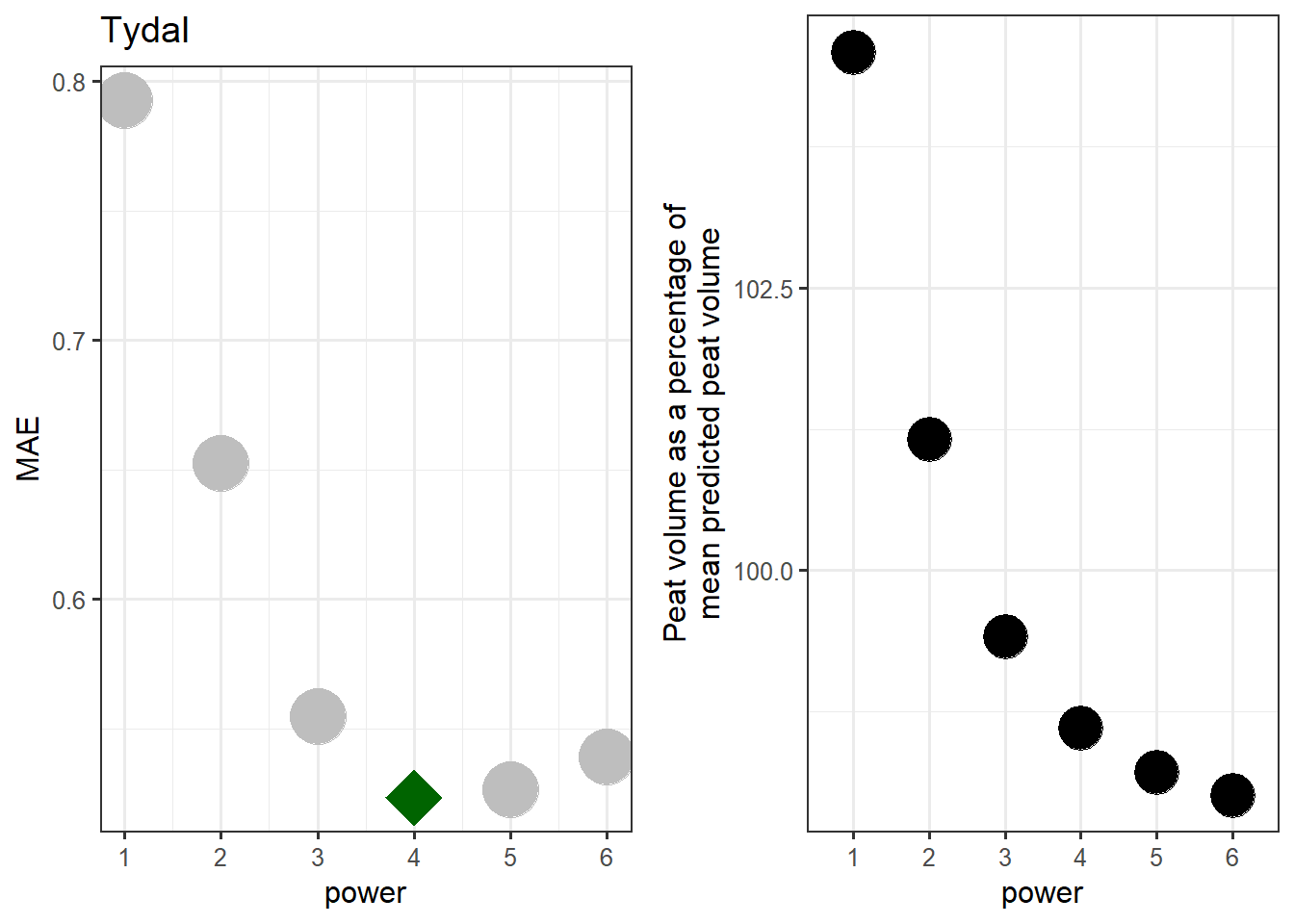
Figure 5.2: Determening the optimal power setting for IDW using a reduced dataset from the Tydal test site.
That’s good. The optimum power is the same as when we had all the data points.
Let’s plot the IDW predictions for Tydal based on all the data pionts and based on the reduced set of data points.
IDW_tydal_4_red <- gstat::idw(formula = Dybde ~ 1,
    locations = depths_tydal_i60, newdata = grid_Tydal_stars_crop,
    idp = 4, nmax = nmax)
#> [inverse distance weighted interpolation]
tm_tydal_red <- tm_shape(IDW_tydal_4_red) + tm_raster(col = "var1.pred",
    palette = "-viridis", title = "Interpolated peat\ndepth (m)") +
    tm_shape(depths_tydal_i60) + tm_symbols(shape = 4,
    col = "black", size = 0.5) + tm_compass(type = "8star",
    position = c("right", "bottom"), size = 2) + tm_scale_bar(position = c("left",
    "bottom"), width = 0.3) + tm_layout(inner.margins = c(0.15,
    0.05, 0, 0.05), legend.outside = T)

tmap_arrange(tm_tydal, tm_tydal_red)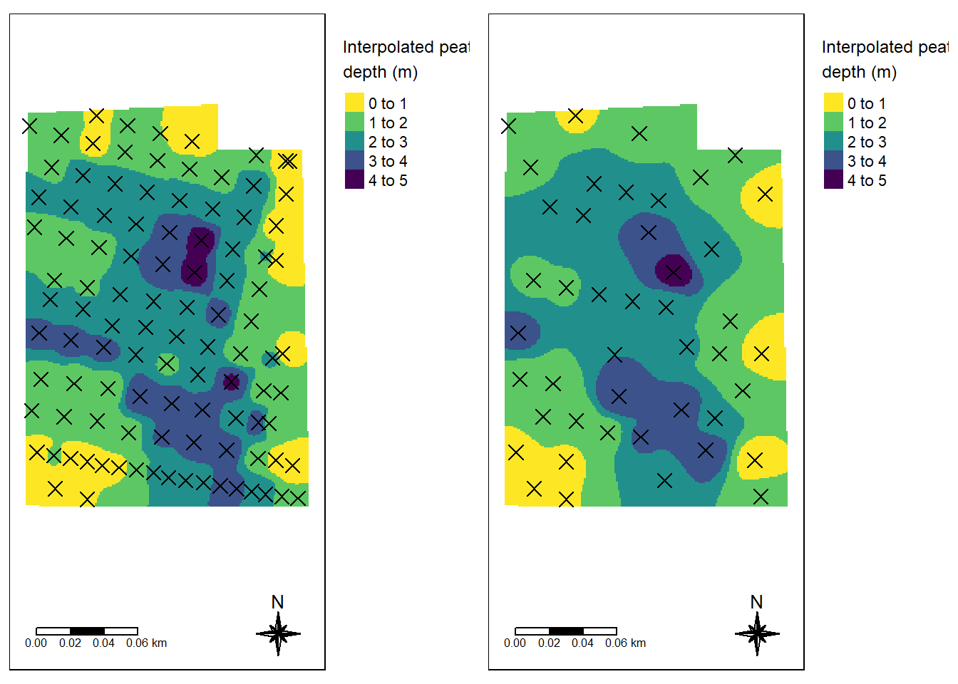
Figure 5.3: Comparing IDW prediction using all data points (left) and a reduced set of data points with median distance between point set to 20 meters.
The two maps in Fig. 5.3 are qualitatively similar.