6 Carbon stocks
Now I want to convert the peat volumes into estimates of carbon stock. This conversion depends on the values of some peat characteristics, such as bulk density and C concentrations. We have a data set with these values.
Import dataset with peat characteristics.
peatCharacteristics <- read_delim("Data/peatCharacteristics.csv",
    delim = ";", escape_double = FALSE, locale = locale(encoding = "ISO-8859-1"),
    trim_ws = TRUE)
dim(peatCharacteristics)
#> [1] 88 30
Each sample consists of multiple sub samples from different depths. Here we will ignore the depth aspect, and simply take the mean from each sample core. This part of the analyses can be improved.
peatCharacteristics_summedDepths <- peatCharacteristics %>%
    mutate(perc_SOM = as.numeric(`% SOM`)) %>%
    mutate(BD = as.numeric(`BD (t/m3)`)) %>%
    dplyr::select(`SAMPLE ID2`, perc_SOM, BD) %>%
    group_by(`SAMPLE ID2`) %>%
    summarise(across(.fns = list(mean = ~mean(., na.rm = TRUE))))

# Getting the other variables that I also want to
# keep
df_info <- peatCharacteristics %>%
    dplyr::select(`SAMPLE ID2`, `General Peatland Type`,
        `Specific Peatland Type`) %>%
    group_by(`SAMPLE ID2`) %>%
    unique()
# and join together again (this two-stap
# proceedure could be simplified)
df = full_join(peatCharacteristics_summedDepths, df_info,
    by = "SAMPLE ID2") %>%
    drop_na()
head(df)
#> # A tibble: 6 x 5
#>   `SAMPLE ID2` perc_SOM_mean BD_mean General Peatl~1 Speci~2
#>   <chr>                <dbl>   <dbl> <chr>           <chr>
#> 1 0029                  98.3  0.05   fen             poor f~
#> 2 0030                  99.5  0.102  fen             interm~
#> 3 0031                  98.2  0.0527 bog             bog
#> 4 0032                  95.9  0.0555 fen             poor f~
#> 5 0033                  96.6  0.067  fen             interm~
#> 6 0034                  99.3  0.066  fen             rich f~
#> # ... with abbreviated variable names
#> #   1: `General Peatland Type`, 2: `Specific Peatland Type`
We have 12 samples from bogs, and 14 from fens:
table(df$`General Peatland Type`)
#>
#> bog fen
#>  12  14
We do not perhaps have enough data points to really compare the different specific peatland types:
table(df$`Specific Peatland Type`)
#>
#>              bog intermediate fen      oceanic bog
#>                3                5                2
#>         poor fen       raised bog         rich fen
#>                5                7                4
Let’s get the total peat volumes for Tydal (and Geilo, but I will not look at Geilo here).
volume
#>    site    volume
#> 1 Tydal  77336.97
#> 2 Geilo 102469.96
Calculating the c stocks (tons C) for the Tydal site without specifying the mire type
c_stock_tydal_uninformed <- volume$volume[volume$site ==
    "Tydal"] * mean(df$perc_SOM_mean/100) * mean(df$BD_mean) *
    0.5  #* 1000 # removing the original conversion from tons to kg
c_stock_tydal_uninformed
#> [1] 3519.665
I think we also need to estimate the uncertainties around this number. Note that for the peat volume estimation, we did not calculate an uncertainty. But for the peat characteristics we have an uncertainty in therms of variation within and between samples points. I will calculate the uncertainty between individual peat cores only.
c_stock_tydal_uninformed <- NULL
for (i in 1:1000) {
    temp <- volume$volume[volume$site == "Tydal"] *
        mean(sample(df$perc_SOM_mean, replace = T)/100) *
        mean(sample(df$BD_mean, replace = T) * 0.5)

    c_stock_tydal_uninformed <- c(c_stock_tydal_uninformed,
        temp)
}
hist(c_stock_tydal_uninformed, main = "", xlab = "C stock")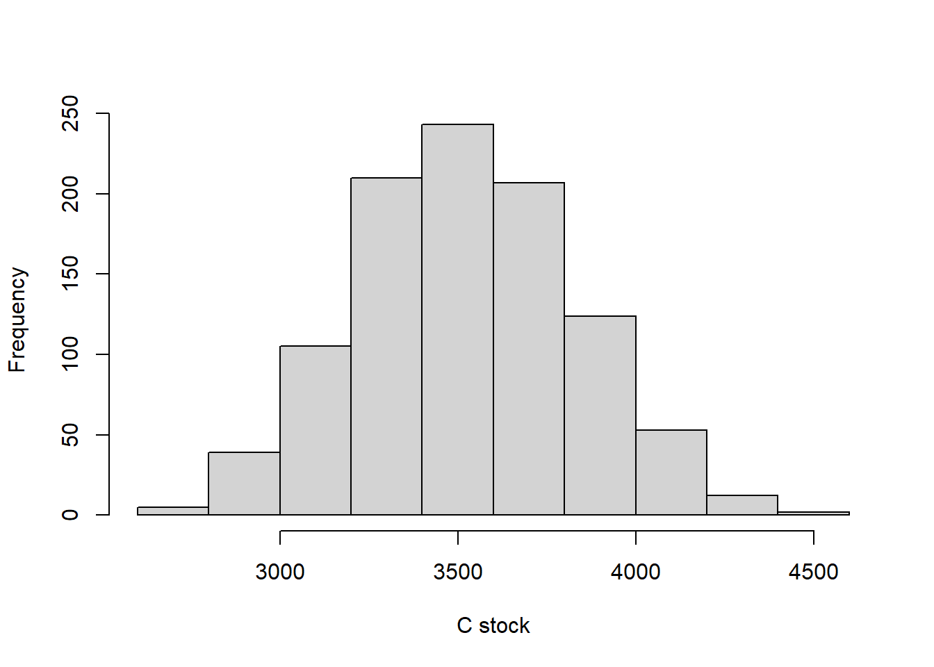
Figure 6.1: Estaimted carbon stock in the Tydal peatland
This distribution is quite wide. Let’s summarize the distribution.
c(quantile(c_stock_tydal_uninformed, c(0.05, 0.5, 0.95)),
    mean = mean(c_stock_tydal_uninformed), sd = sd(c_stock_tydal_uninformed))
#>        5%       50%       95%      mean        sd
#> 3027.9073 3528.9171 4022.0120 3526.0560  307.4721
We can put this stuff into a more generic function.
ccalc_cStocks <- function(volume, peatlandType = c("fen",
    "bog"), peatData) {
    temp_stocks <- NULL
    temp_peatData <- peatData[peatData$`General Peatland Type` %in%
        peatlandType, ]

    for (i in 1:1000) {
        temp <- volume * mean(sample(peatData$perc_SOM_mean,
            replace = T)/100) * mean(sample(peatData$BD_mean,
            replace = T) * 0.5)

        temp_stocks <- c(temp_stocks, temp)
    }
    return(c(quantile(temp_stocks, c(0.05, 0.5, 0.95)),
        mean = mean(temp_stocks), sd = sd(temp_stocks)))
}
Calculating summary statistics for the carbon stocks in Tydal, using both general peatland types.
(cstocks_tydal_unspecified <- ccalc_cStocks(volume = volume$volume[volume$site ==
    "Tydal"], peatData = df))
#>        5%       50%       95%      mean        sd
#> 3020.5840 3508.5842 4006.3984 3513.4878  307.8291
And using only the bog data.
(cstocks_tydal_bog <- ccalc_cStocks(volume = volume$volume[volume$site ==
    "Tydal"], peatData = df, peatlandType = "bog"))
#>        5%       50%       95%      mean        sd
#> 3003.8746 3519.8539 4052.2213 3524.2160  313.0933
And finally, aslo the fen data.
(cstocks_tydal_fen <- ccalc_cStocks(volume = volume$volume[volume$site ==
    "Tydal"], peatData = df, peatlandType = "fen"))
#>        5%       50%       95%      mean        sd
#> 3034.1716 3528.3966 4036.1386 3524.4508  309.0369
cstocks_tydal_unspecified_df <- as.data.frame(cstocks_tydal_unspecified)
names(cstocks_tydal_unspecified_df) <- "C stocks"
cstocks_tydal_unspecified_df$summary <- row.names(cstocks_tydal_unspecified_df)
cstocks_tydal_unspecified_df$information <- "Unspecified"


cstocks_tydal_bog_df <- as.data.frame(cstocks_tydal_bog)
names(cstocks_tydal_bog_df) <- "C stocks"
cstocks_tydal_bog_df$summary <- row.names(cstocks_tydal_bog_df)
cstocks_tydal_bog_df$information <- "Bog"

cstocks_tydal_fen_df <- as.data.frame(cstocks_tydal_fen)
names(cstocks_tydal_fen_df) <- "C stocks"
cstocks_tydal_fen_df$summary <- row.names(cstocks_tydal_fen_df)
cstocks_tydal_fen_df$information <- "Fen"

cstocks_tydal_compare <- rbind(cstocks_tydal_fen_df,
    cstocks_tydal_bog_df, cstocks_tydal_unspecified_df)

# Pivot
cstocks_tydal_compare <- pivot_wider(cstocks_tydal_compare,
    names_from = summary, values_from = "C stocks")
(tmp_out <- ggplot(cstocks_tydal_compare, aes(x = information)) +
    geom_point(aes(y = mean), shape = 15, size = 10) +
    geom_linerange(aes(ymin = `5%`, ymax = `95%`),
        size = 2) + theme_bw(base_size = 16) + labs(x = "Peat characteristics",
    y = "Carbon stocks (tons)"))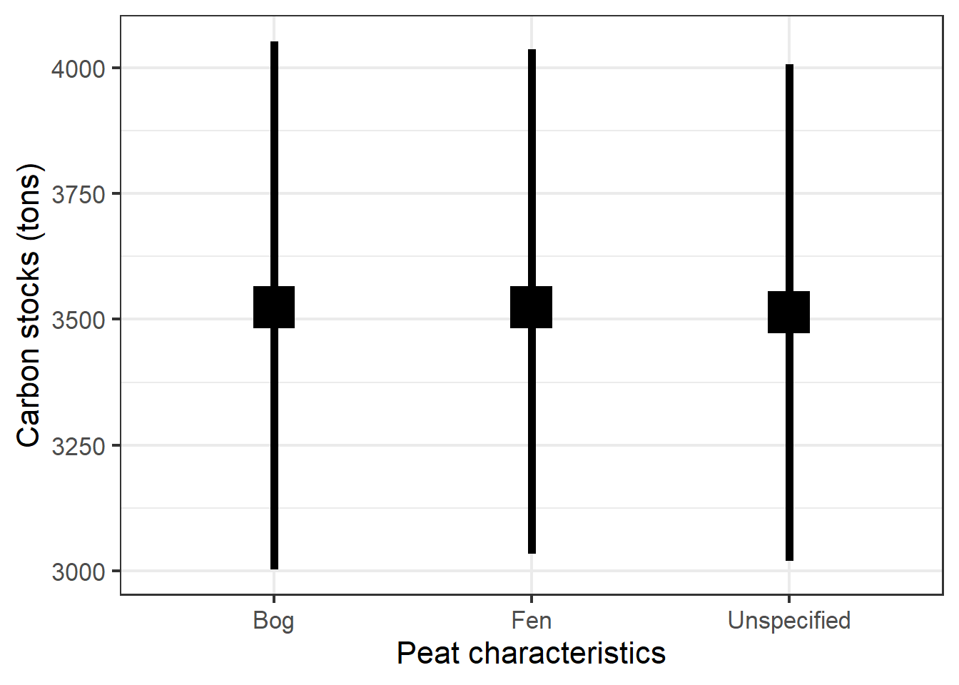
Figure 6.2: Mean (± 95 CI) carbon stock for the Tydal test site.
Specifying the peatland type makes no difference!
Let’s just get the (non-informed) C stock estimates for Geilo as well
ccalc_cStocks(volume = volume$volume[volume$site ==
    "Geilo"], peatData = df)
#>        5%       50%       95%      mean        sd
#> 3973.0322 4654.0340 5361.8161 4652.9012  421.2738