2 Test data

2.1 Peat depth and peatland delineation

To create the methodology for mapping peatland depth profiles, and estimating peat volume, carbon stocks and sensitivity to sampling effort, I will use two contrasting test sites: Tydal and Geilo. Later, in chapter 7 I will validate the generality of this method on an additional four sites. For more details on the justification and the methods used, please the manuscript.

Libraries used:

library(tmap)
library(sf)
library(readr)
library(tmaptools)
library(basemaps)
library(ggplot2)
library(ggpubr)
library(gstat)
library(matrixStats)
library(ggtext)
library(tidyverse)
library(osmplotr)

Import shape files with peatland delineations and fix the coordinate reference system (CRS).

SHP_tydal <- sf::read_sf("Data/Tydal/stasjon_Setermyra.shp")
SHP_geilo <- sf::read_sf("Data/Geilo/geilo-dybdef.shp")

# st_crs(SHP_tydal) st_crs(SHP_geilo)# NA I found
# CRS through trial and error. It is UTM 32
st_crs(SHP_geilo) <- 25832

# Transform to UTM33N
SHP_geilo <- st_transform(SHP_geilo, 25833)

Import peat depth measurements for the two sites.

depths_tydal <- readr::read_csv("Data/Tydal/Torvdybder_Tydal_stasjon.csv")
depths_geilo <- read.csv("Data/Geilo/torvdybder.csv",
    sep = ";")


# convert data.frames to simple features.
depths_tydal <- sf::st_as_sf(x = depths_tydal, coords = c("coords.x1",
    "coords.x2"), crs = "+init=epsg:25833")
depths_geilo <- st_as_sf(x = depths_geilo, coords = c("x",
    "y"), crs = "+init=epsg:25832")

# Tranbsform to UTM33, same as the shape file
depths_geilo <- st_transform(depths_geilo, 25833)

# Confirm overlap. Using base plotting to avoid
# auto-transformation
plot(SHP_geilo$geometry, col = "red")
plot(depths_geilo$geometry, pch = 16, col = "grey",
    cex = 0.1, add = T)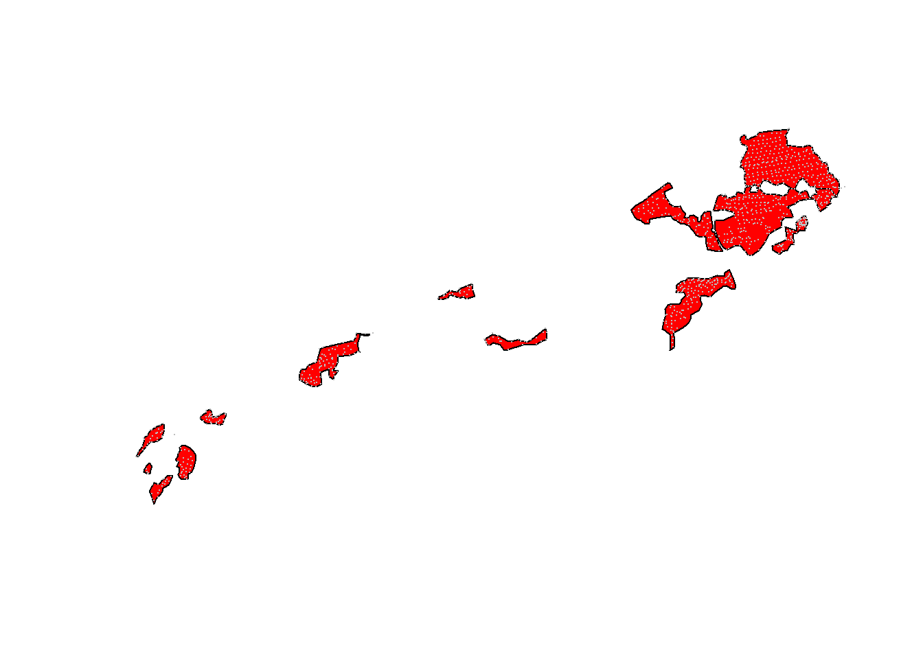

Figure 2.1: Confirming overlap between shape file and depth measurements

That looks fine.

Download basemaps for some context.

# osmplotr want bboxes in latlong
SHP_geilo_ll <- sf::st_transform(SHP_geilo, 4326)
SHP_tydal_ll <- sf::st_transform(SHP_tydal, 4326)

bb_Geilo <- sf::st_bbox(SHP_geilo_ll)
bb_Tydal <- sf::st_bbox(SHP_tydal_ll)

# GEILO
base_geilo_hw <- osmplotr::extract_osm_objects(bbox = bb_Geilo,
    key = c("highway"), sf = T)
base_geilo_building <- osmplotr::extract_osm_objects(bbox = bb_Geilo,
    key = c("building"), sf = T)
base_geilo_ww <- osmplotr::extract_osm_objects(bbox = bb_Geilo,
    key = c("waterway"), sf = T, return_type = "line")

# TYDAL
base_tydal_hw <- osmplotr::extract_osm_objects(bbox = bb_Tydal,
    key = "highway", sf = T)
base_tydal_building <- osmplotr::extract_osm_objects(bbox = bb_Tydal,
    key = c("building"), sf = T)
base_tydal_ww <- osmplotr::extract_osm_objects(bbox = bb_Tydal,
    key = c("waterway"), sf = T, return_type = "line")

Plot static map

# GEILO
static_geilo <- tm_shape(SHP_geilo_ll) + tm_polygons(col = "green") +
    tm_shape(depths_geilo) + tm_dots() + tm_shape(base_geilo_hw) +
    tm_lines() + tm_shape(base_geilo_ww) + tm_lines(col = "blue",
    size = 2) + tm_shape(base_geilo_building) + tm_polygons(col = "black",
    alpha = 0.3) + tm_compass() + tm_scale_bar() +
    tm_layout(title = "Geilo")


# TYDAL
static_tydal <- tm_shape(SHP_tydal_ll) + tm_polygons(col = "green") +
    tm_shape(depths_tydal) + tm_dots(size = "Dybde",
    col = "Dybde", palette = "-viridis") + tm_shape(base_tydal_ww) +
    tm_lines(col = "blue", size = 2) + tm_compass() +
    tm_scale_bar() + tm_layout(title = "Tydal", legend.show = F,
    inner.margins = c(0.1, 0.02, 0.1, 0.02))

tmap_arrange(static_geilo, static_tydal)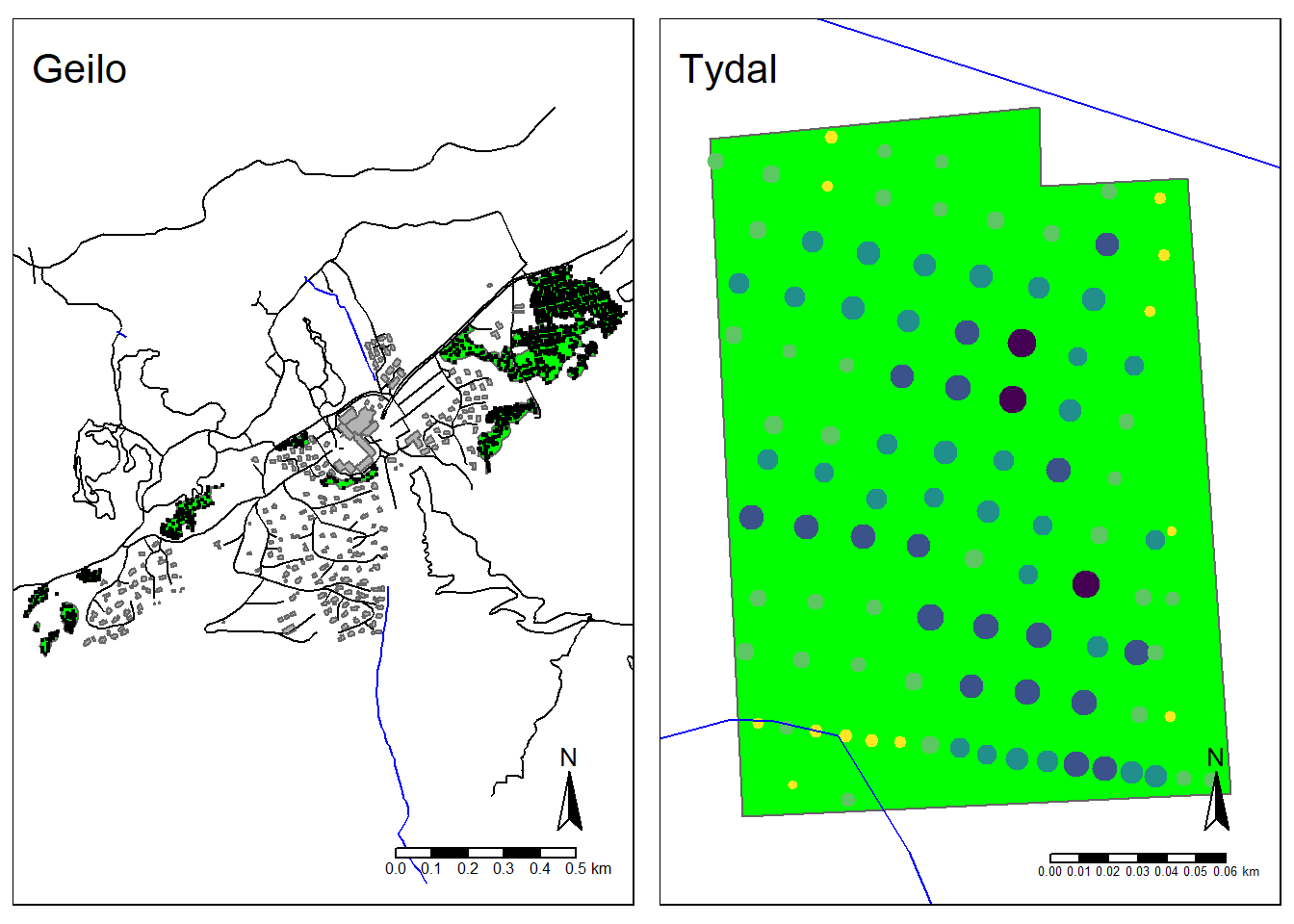

Figure 2.2: Map of Geilo and Tydal test sites. The peatland is deliminated as a green polygon(s). Dots are depth measurements and for Tydal the colour and size of the dots reflects the measured peat depths in meters.

These two test cases are very different. Geilo is a set of several unique mire polygons. Usually, in development projects, one would estimate the peat volume and C stock for each of these separately, but we will try now to see if it can be done in one operation. Tydal is a more typical example of a clear peatland delineation. Both cases have dense peat depth measurements taken.