7 Additional test sites
We used two contrasting sites, Tydal and Geilo, for the main analyses and testing. Now I will bring in an additional four sites to validate the generality of these finding.
7.1 Modalen
Import shape files with peatland delineations.
SHP_modalen <- sf::read_sf("Data/Modalen/Modalen_myrareal.shp")
# st_crs(SHP_modalen) #OK
Another shape file with the project area (see below)
SHP_modalen_project <- sf::read_sf("Data/Modalen/modalen_shp.shp")
# st_crs(SHP_modalen_project) # OK
Import depth samples
depths_modalen <- sf::read_sf("Data/Modalen/modalen_punkter.shp")
# st_crs(depths_modalen) #OK
tm_shape(SHP_modalen) + tm_polygons() + tm_shape(depths_modalen) +
    tm_symbols(col = "black", size = 0.5, shape = 4) +
    tm_shape(SHP_modalen_project) + tm_borders(lty = "dotted") +
    tm_compass(type = "8star", position = c("right",
        "bottom"), size = 2) + tm_scale_bar(position = c("left",
    "bottom"), width = 0.3) + tm_layout(inner.margins = c(0.15,
    0.05, 0.05, 0.05))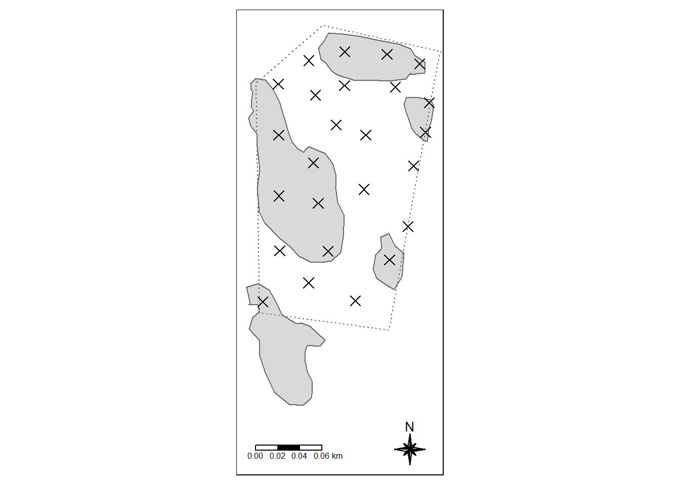
Figure 7.1: The Modalen test site sith peatland delineated as grey polygons. Crosses are peat depth samples, contained with in the project area (dotted line).
The peatland delineation (five peatlands inside the project area) is mapped using aerial photos and other base maps. There may be peat also between these polygons, however, there is for sure areas between the polygons that are not peat. The depth measurements are performed systematically inside the project area. I don’t think we should include points that are taken from smaller isolated mire fragments that are clearly separated from the main peatlands. This example illustrates the importance of appropriate sampling. We are now limited to just a few data points. The smaller mires have only one or two data points.
Calculating the combined area of the five mires.
And the area of the project delineation
SHP_modalen_project$myArea <- sf::st_area(SHP_modalen_project)
SHP_modalen_project$myArea
#> 36179.43 [m^2]
Removing the depth measurement from outside the peatland delinitaion
depths_modalen_reduced <- sf::st_intersection(depths_modalen,
    SHP_modalen)
#> Warning: attribute variables are assumed to be spatially
#> constant throughout all geometries
tm_shape(SHP_modalen) + tm_polygons() + tm_shape(depths_modalen_reduced) +
    tm_symbols(col = "black", size = 0.5, shape = 4) +
    tm_shape(SHP_modalen_project) + tm_borders(lty = "dotted") +
    tm_compass(type = "8star", position = c("right",
        "bottom"), size = 2) + tm_scale_bar(position = c("left",
    "bottom"), width = 0.3) + tm_layout(inner.margins = c(0.15,
    0.05, 0.05, 0.05))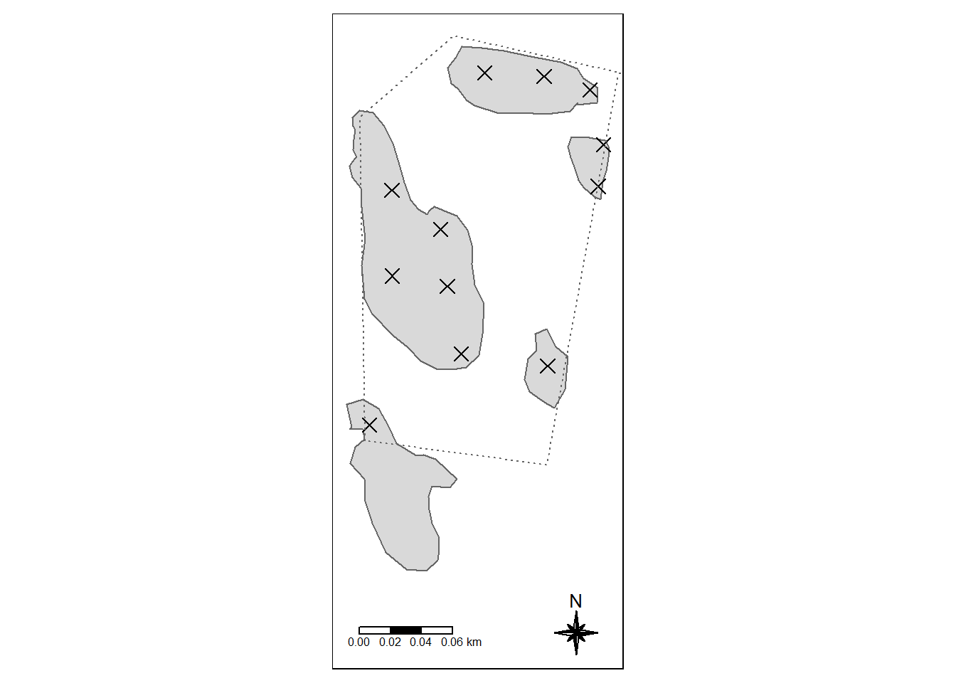
Figure 7.2: The Modalen test site sith peatland delineated as grey polygons. Crosses are peat depth samples, contained with in the project area (dotted line). Only depth measurements that intersects the mire polygons are included
Create a raster grid
# First fix polygon closure
SHP_modalen <- sf::st_make_valid(SHP_modalen)


grid_Modalen_stars_crop <- starsExtra::make_grid(SHP_modalen,
    1) %>%
    sf::st_crop(SHP_modalen)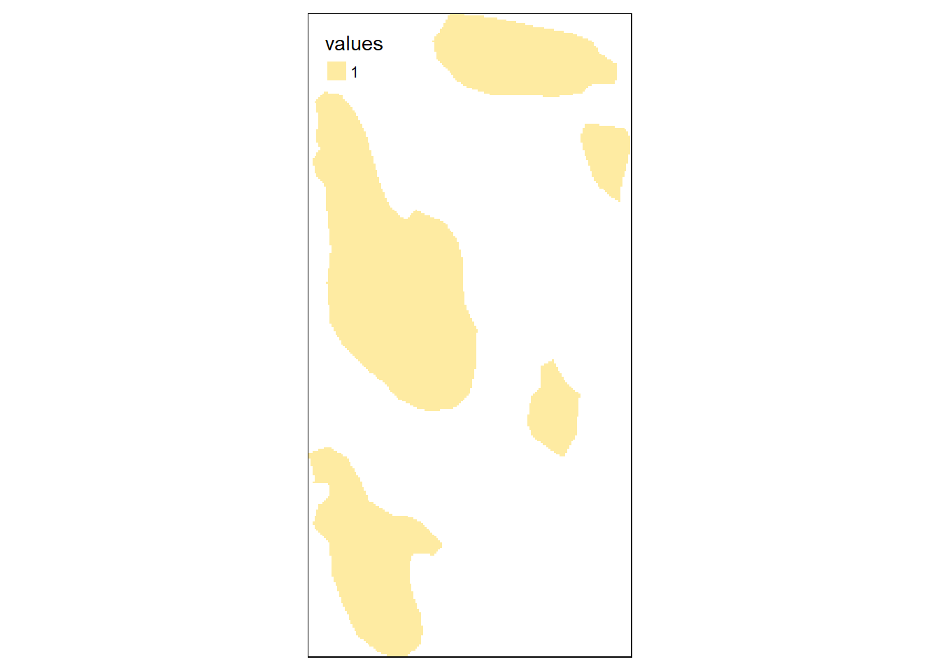
Figure 7.3: Checking that the raster grid for Modalen looks correct.
Predict peat depth
ccalc_optimumPower(nmax = nrow(depths_modalen_reduced),
    peatDepths = depths_modalen_reduced, title = "Modalen",
    peatlandDelimination = SHP_modalen)
#>
  |
  |                                                  |   0%
  |
  |=====                                             |   9%
  |
  |=========                                         |  18%
  |
  |==============                                    |  27%
  |
  |==================                                |  36%
  |
  |=======================                           |  45%
  |
  |===========================                       |  55%
  |
  |================================                  |  64%
  |
  |====================================              |  73%
  |
  |=========================================         |  82%
  |
  |=============================================     |  91%
  |
  |==================================================| 100%
#> [inverse distance weighted interpolation]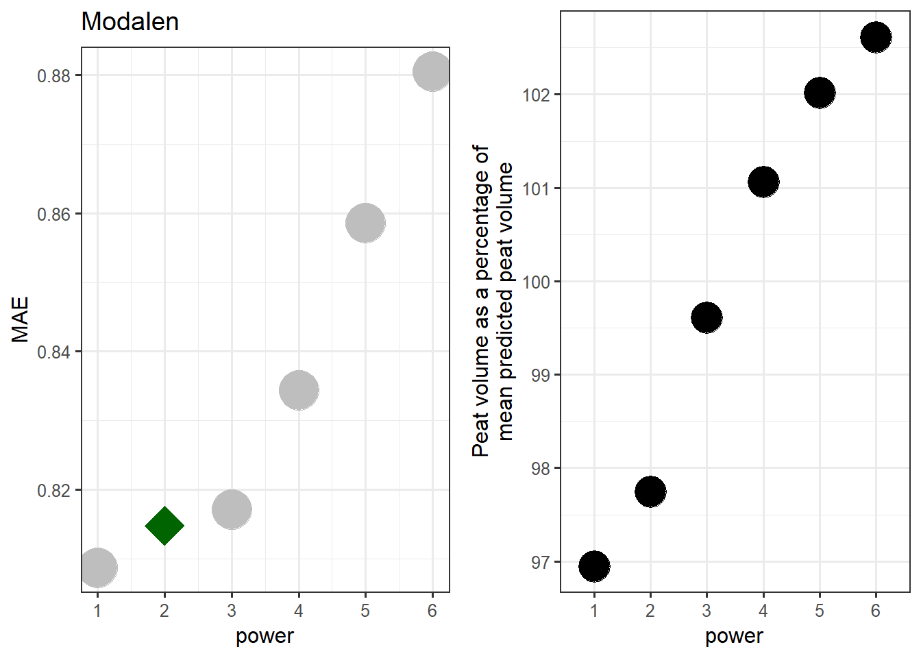
Figure 7.4: Determening the optimal power for the Modelan test site.
Unsurprising, when we have so few data points, the optimum power is very low. I will predict using power 1 through 3 to compare, just because I don’t trust power 1 is the best choice.
IDW_Modalen_1 <- gstat::idw(formula = Dybde ~ 1, locations = depths_modalen_reduced,
    newdata = grid_Modalen_stars_crop, idp = 1, nmax = 20)  # nmax > than the number of points
#> [inverse distance weighted interpolation]

IDW_Modalen_2 <- gstat::idw(formula = Dybde ~ 1, locations = depths_modalen_reduced,
    newdata = grid_Modalen_stars_crop, idp = 2, nmax = nrow(depths_modalen_reduced))
#> [inverse distance weighted interpolation]

IDW_Modalen_3 <- gstat::idw(formula = Dybde ~ 1, locations = depths_modalen_reduced,
    newdata = grid_Modalen_stars_crop, idp = 3, nmax = nrow(depths_modalen_reduced))
#> [inverse distance weighted interpolation]
tmap_arrange(
tm_shape(IDW_Modalen_1)+
  tm_raster(col="var1.pred",
            palette = "-viridis",
            title = "Power = 1\nInterpolated peat\ndepth (m)",
            breaks = seq(0,3,.5))+
  tm_compass(type="8star", position = c("right", "bottom"), size = 2) +
  tm_scale_bar(position = c("right", "bottom"), width = 0.3)+
  tm_shape(depths_modalen_reduced)+
  tm_symbols(shape=4,
             col="black",
             size=.5)+
  tm_layout(legend.outside = T)
,
tm_shape(IDW_Modalen_2)+
  tm_raster(col="var1.pred",
            palette = "-viridis",
            title = "Power = 2\nInterpolated peat\ndepth (m)",
            breaks = seq(0,3,.5))+
  tm_compass(type="8star", position = c("right", "bottom"), size = 2) +
  tm_scale_bar(position = c("right", "bottom"), width = 0.3)+
  tm_shape(depths_modalen_reduced)+
  tm_symbols(shape=4,
             col="black",
             size=.5)+
  tm_layout(legend.outside = T)
,
tm_shape(IDW_Modalen_3)+
  tm_raster(col="var1.pred",
            palette = "-viridis",
            title = "Power = 3\nInterpolated peat\ndepth (m)",
            breaks = seq(0,3,.5))+
  tm_compass(type="8star", position = c("right", "bottom"), size = 2) +
  tm_scale_bar(position = c("right", "bottom"), width = 0.3)+
  tm_shape(depths_modalen_reduced)+
  tm_symbols(shape=4,
             col="black",
             size=.5)+
  tm_layout(legend.outside = T)

)
#> Legend labels were too wide. The labels have been resized to 0.46, 0.46, 0.46, 0.46, 0.46, 0.46. Increase legend.width (argument of tm_layout) to make the legend wider and therefore the labels larger.
#> Legend labels were too wide. The labels have been resized to 0.46, 0.46, 0.46, 0.46, 0.46, 0.46. Increase legend.width (argument of tm_layout) to make the legend wider and therefore the labels larger.
#> Legend labels were too wide. The labels have been resized to 0.46, 0.46, 0.46, 0.46, 0.46, 0.46. Increase legend.width (argument of tm_layout) to make the legend wider and therefore the labels larger.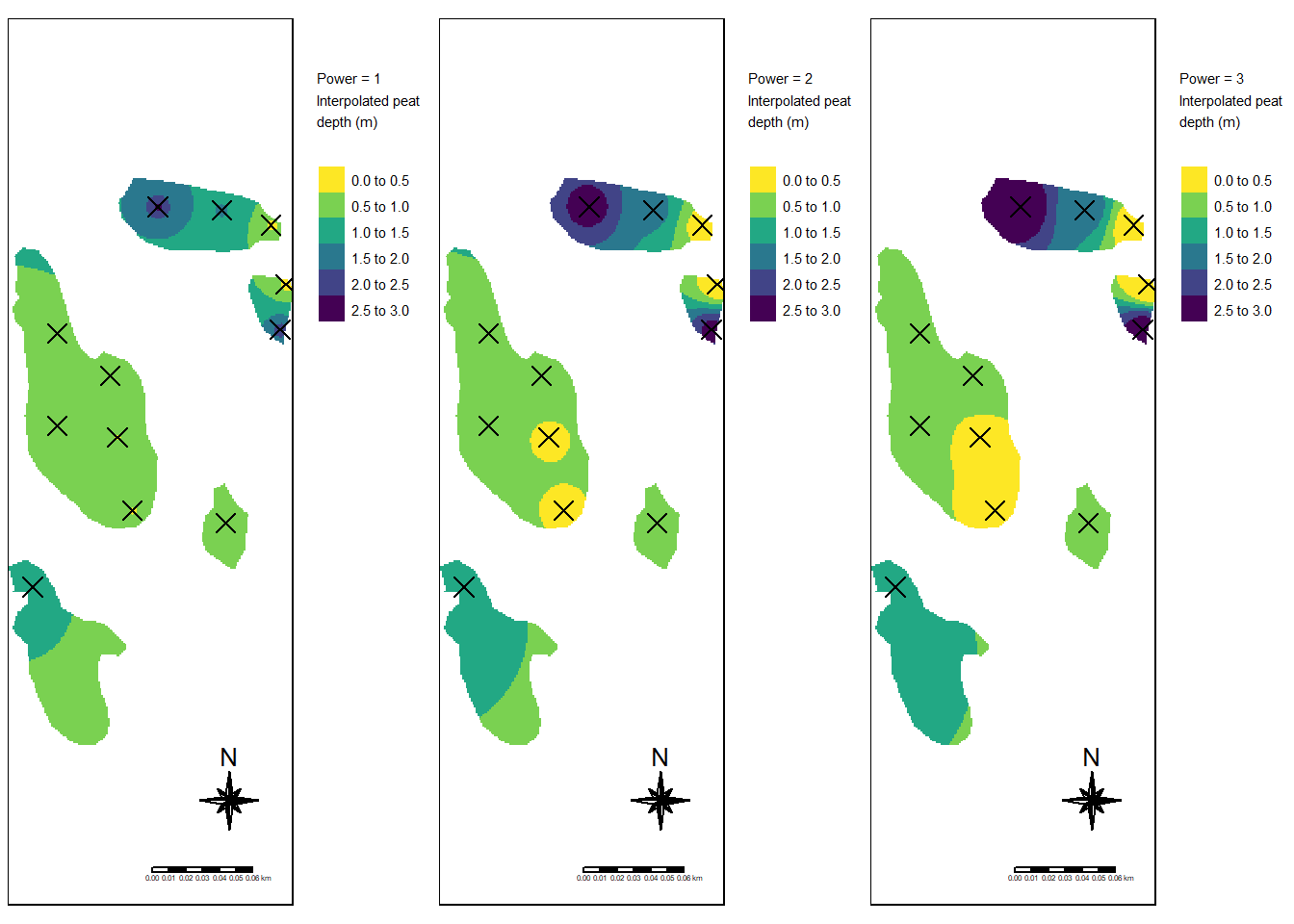
Figure 7.5: IDW for peat depth at Modalen test site.
I think power 3 looks more accurate because of the way it gives weight to local points. The recommended practice for this case I think would be to analyse each polygon or mire separately because of how the point from neighboring mires affect the depth predictions.
Summary stats for the peat depth at Modalen.
summary(depths_modalen_reduced$Dybde)
#>    Min. 1st Qu.  Median    Mean 3rd Qu.    Max.
#>   0.000   0.400   0.600   1.017   1.475   2.800
The MAE for the power =3 prediction is 0.82 m.
The rough volume (in m3), that is the mean peat depth multiplied by the area, is
Number of depth samples per 100 m2:
12/(sum(SHP_modalen$myArea)/100)
#> 0.07163001 [1/m^2]
Interpolated volume
(volume_modalen <- sum(IDW_Modalen_3$var1.pred, na.rm = T))
#> [1] 16792.6
Estimated carbon stocks for the Modalen site:
ccalc_cStocks(volume_modalen, peatData = df)
#>        5%       50%       95%      mean        sd
#> 641.03119 760.77403 876.66458 759.42009  69.07228
7.2 Opelandsmarka
Import shape file
SHP_opelandsmarka <- sf::read_sf("Data/Opelandsmarka/Opelandsmarka Voss.shp")
# st_crs(SHP_opedalsmarka) #32632 UTM 32
The depth measurements are in three different files.
depths_opelandsmarka1 <- read_delim("Data/Opelandsmarka/Torvdybder_Opelandsmarka_myr1.csv",
    delim = ";", escape_double = FALSE, locale = locale(encoding = "ISO-8859-1"),
    trim_ws = TRUE)
depths_opelandsmarka2 <- read_delim("Data/Opelandsmarka/Torvdybder_Opelandsmarka_myr2.csv",
    delim = ";", escape_double = FALSE, locale = locale(encoding = "ISO-8859-1"),
    trim_ws = TRUE)
depths_opelandsmarka3 <- read_delim("Data/Opelandsmarka/Torvdybder_Opelandsmarka_myr3.csv",
    delim = ";", escape_double = FALSE, locale = locale(encoding = "ISO-8859-1"),
    trim_ws = TRUE)
# The last one is missing a column

depths_opelandsmarka <- bind_rows(depths_opelandsmarka1,
    depths_opelandsmarka2, depths_opelandsmarka3)


depths_opelandsmarka <- sf::st_as_sf(depths_opelandsmarka,
    coords = c("UTM_N_ZONE32N", "UTM_E_ZONE32N"), crs = 32632)
tm_shape(SHP_opelandsmarka) + tm_polygons() + tm_shape(depths_opelandsmarka) +
    tm_symbols(col = "black", size = 0.5, shape = 4)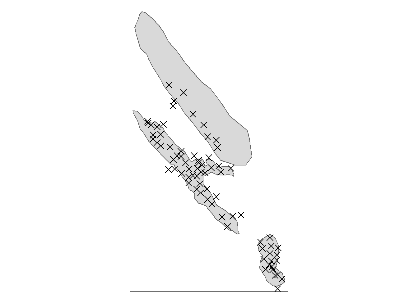
Figure 7.6: Test site: Opelandsmarka. Crosses are peat depth measurements.
I think we can ignore that top mire as it was not sampled nearly as intensive as the other two.
SHP_opelandsmarka_twoMires <- SHP_opelandsmarka[-1,
    ]
It could be a good idea sometimes to include depth measurements outside the mire polygons (with a depth of 0). Here it is easier for me to just exclude all points outide any polygon.
depths_opelandsmarka <- st_intersection(depths_opelandsmarka,
    SHP_opelandsmarka_twoMires)
#> Warning: attribute variables are assumed to be spatially
#> constant throughout all geometries
tm_shape(SHP_opelandsmarka_twoMires) + tm_polygons() +
    tm_shape(depths_opelandsmarka) + tm_symbols(col = "black",
    size = 0.5, shape = 4)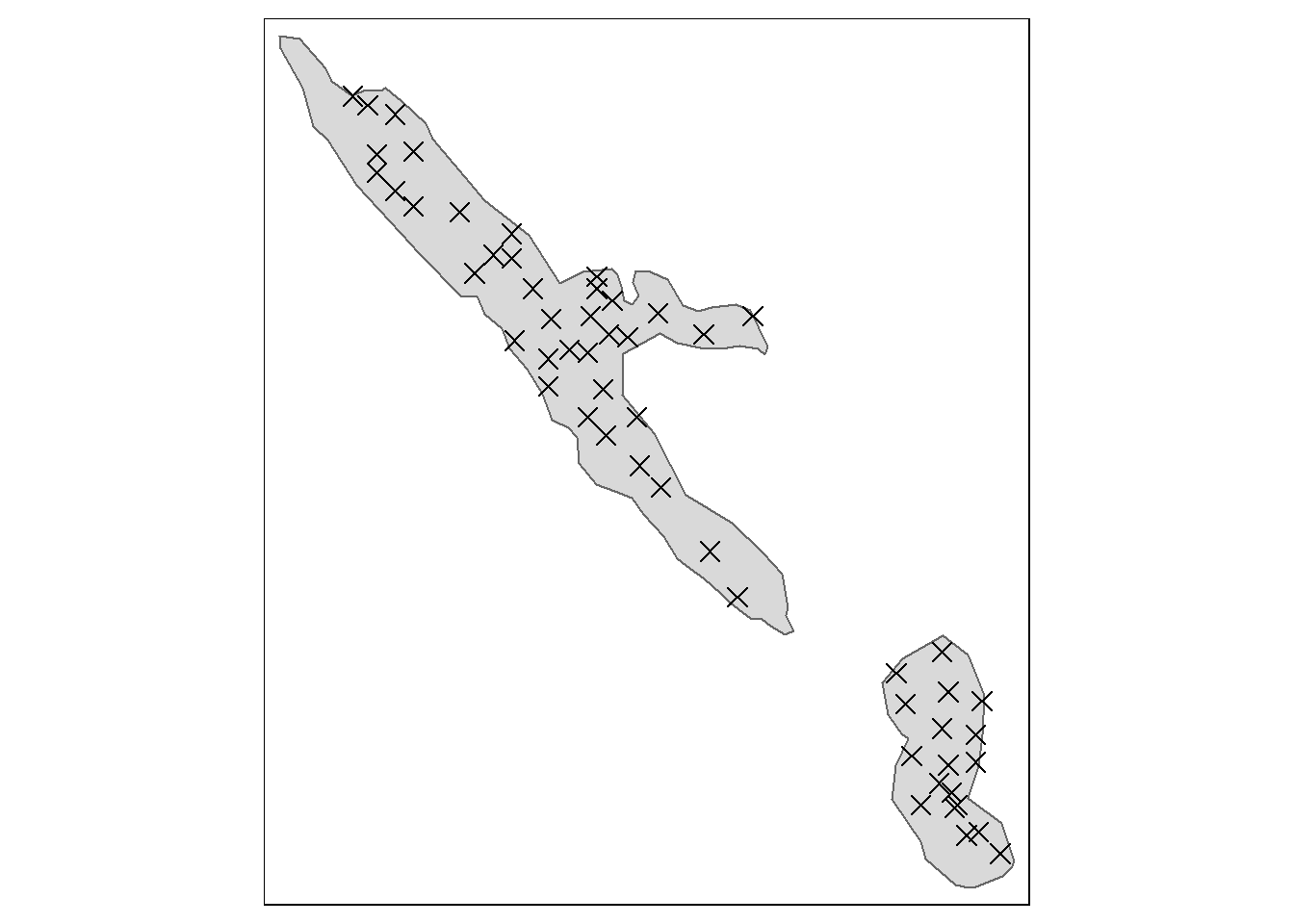
Figure 7.7: Opelandsmarka with two out of three mires. Crosses are peat depth measurements.
There is one NA in the depth data which we have to remove
depths_opelandsmarka <- depths_opelandsmarka[!is.na(depths_opelandsmarka$Dybde),
    ]
Try again:
ccalc_optimumPower(peatDepths = depths_opelandsmarka,
title = "Opelandsmarka", peatlandDelimination = SHP_opelandsmarka_twoMires)
#>
|
| | 0%
|
|= | 2%
|
|== | 4%
|
|=== | 6%
|
|==== | 8%
|
|===== | 9%
|
|====== | 11%
|
|======= | 13%
|
|======== | 15%
|
|======== | 17%
|
|========= | 19%
|
|========== | 21%
|
|=========== | 23%
|
|============ | 25%
|
|============= | 26%
|
|============== | 28%
|
|=============== | 30%
|
|================ | 32%
|
|================= | 34%
|
|================== | 36%
|
|=================== | 38%
|
|==================== | 40%
|
|===================== | 42%
|
|====================== | 43%
|
|======================= | 45%
|
|======================== | 47%
|
|========================= | 49%
|
|========================= | 51%
|
|========================== | 53%
|
|=========================== | 55%
|
|============================ | 57%
|
|============================= | 58%
|
|============================== | 60%
|
|=============================== | 62%
|
|================================ | 64%
|
|================================= | 66%
|
|================================== | 68%
|
|=================================== | 70%
|
|==================================== | 72%
|
|===================================== | 74%
|
|====================================== | 75%
|
|======================================= | 77%
|
|======================================== | 79%
|
|========================================= | 81%
|
|========================================== | 83%
|
|========================================== | 85%
|
|=========================================== | 87%
|
|============================================ | 89%
|
|============================================= | 91%
|
|============================================== | 92%
|
|=============================================== | 94%
|
|================================================ | 96%
|
|================================================= | 98%
|
|==================================================| 100%
#> [inverse distance weighted interpolation]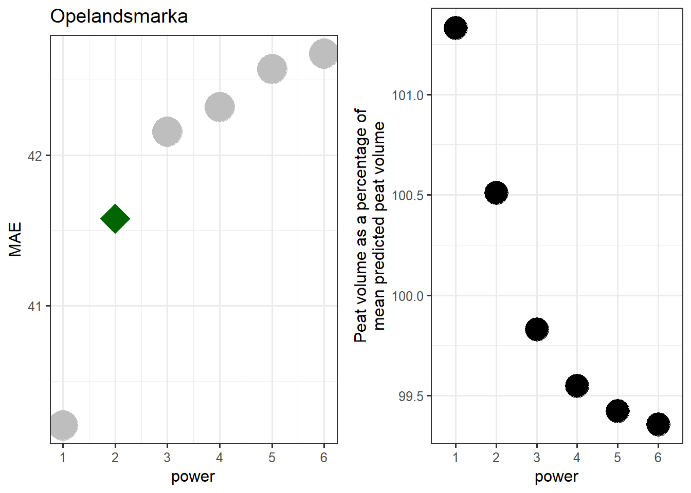
Figure 7.8: Determening the optimal power for the Opelandsmarka test site.
Again the lowest MAE is obtained from a power of 1, but as we have seen, the power should probably be set higher. The predicted peat volume for example is quite unstable at low power settings.
Create a raster grid for the predictions
grid_Opelandsmarka_stars_crop <- starsExtra::make_grid(SHP_opelandsmarka_twoMires,
    1) %>%
    sf::st_crop(SHP_opelandsmarka_twoMires)
The depths are recorded as cm not meters. Converting to m.
depths_opelandsmarka$Dybde <- depths_opelandsmarka$Dybde/100
IDW_opelandsmarka_1 <- gstat::idw(Dybde ~ 1, depths_opelandsmarka,
    newdata = grid_Opelandsmarka_stars_crop, nmax = nmax,
    idp = 1)
#> [inverse distance weighted interpolation]

IDW_opelandsmarka_2 <- gstat::idw(Dybde ~ 1, depths_opelandsmarka,
    newdata = grid_Opelandsmarka_stars_crop, nmax = nmax,
    idp = 2)
#> [inverse distance weighted interpolation]

IDW_opelandsmarka_3 <- gstat::idw(Dybde ~ 1, depths_opelandsmarka,
    newdata = grid_Opelandsmarka_stars_crop, nmax = nmax,
    idp = 3)
#> [inverse distance weighted interpolation]
myBreaks <- seq(0,3,.5)
myPos <- c("left", "bottom")

tmap_arrange(
tm_shape(IDW_opelandsmarka_1)+
  tm_raster(col="var1.pred",
            palette = "-viridis",
            title = "Power = 1\nInterpolated peat\ndepth (m)",
            breaks = myBreaks)+
  tm_compass(type="8star", position = myPos, size = 2) +
  tm_scale_bar(position = myPos, width = 0.3)+
  tm_shape(depths_opelandsmarka)+
  tm_symbols(shape=4,
             col="black",
             size=.5)+
  tm_layout(legend.outside = T)
,
tm_shape(IDW_opelandsmarka_2)+
  tm_raster(col="var1.pred",
            palette = "-viridis",
            title = "Power = 2\nInterpolated peat\ndepth (m)",
            breaks = myBreaks)+
  tm_compass(type="8star", position = myPos, size = 2) +
  tm_scale_bar(position = myPos, width = 0.3)+
  tm_shape(depths_opelandsmarka)+
  tm_symbols(shape=4,
             col="black",
             size=.5)+
  tm_layout(legend.outside = T)
,
tm_shape(IDW_opelandsmarka_3)+
  tm_raster(col="var1.pred",
            palette = "-viridis",
            title = "Power = 3\nInterpolated peat\ndepth (m)",
            breaks = myBreaks)+
  tm_compass(type="8star", position = myPos, size = 2) +
  tm_scale_bar(position = myPos, width = 0.3)+
  tm_shape(depths_opelandsmarka)+
  tm_symbols(shape=4,
             col="black",
             size=.5)+
  tm_layout(legend.outside = T),
ncol = 2

)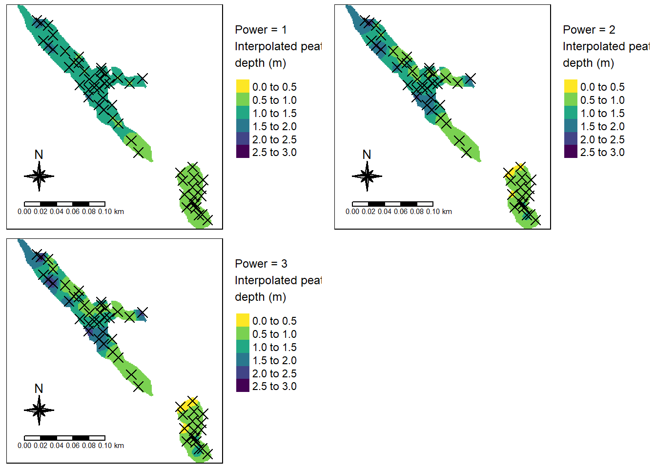
Figure 7.9: Interpolated peat depth at test site Opelandsmarka.
With power set to 1 the model is too flat, and the deep areas are not identified correctly. Power 2 or 3 makes less of a difference. Becaus ethe MAE and volume estimates are so similar, I will chose the modet local model (power = 3)
Getting the total peatland area
SHP_opelandsmarka_twoMires$myArea <- sf::st_area(SHP_opelandsmarka_twoMires)
sum(SHP_opelandsmarka_twoMires$myArea)
#> 8700.213 [m^2]
Getting the mean peat depth (after excluding points outside the polygons)
mean(depths_opelandsmarka$Dybde)
#> [1] 1.058333
Rough volume
Number of peat depth measurements
nrow(depths_opelandsmarka)
#> [1] 54
Depth measurement density (points per 100 m-2)
Interpolated peat volume (best model)
(vol_temp <- sum(IDW_opelandsmarka_3$var1.pred, na.rm = T))
#> [1] 9270.232
Estimated C stocks
ccalc_cStocks(volume = vol_temp, peatData = df)
#>       5%      50%      95%     mean       sd
#> 357.0596 423.1712 485.1275 422.6782  38.0913
7.3 Kinn 1
# import peatland delineation
SHP_kinn1 <- sf::st_read("Data/Kinn/rikmyr_avgrensing.shp")
#> Reading layer `rikmyr_avgrensing' from data source
#>   `C:\Users\anders.kolstad\Github\carbonCalculator\Data\Kinn\rikmyr_avgrensing.shp'
#>   using driver `ESRI Shapefile'
#> Simple feature collection with 1 feature and 27 fields
#> Geometry type: POLYGON
#> Dimension:     XY
#> Bounding box:  xmin: 5.099473 ymin: 61.48336 xmax: 5.102058 ymax: 61.48463
#> Geodetic CRS:  WGS 84

# import peat deth data
depths_kinn1 <- read_delim("Data/Kinn/data_rikmyr_torvdybder.csv",
    delim = ";", escape_double = FALSE, locale = locale(encoding = "ISO-8859-1"),
    trim_ws = TRUE)
The peat depth data doesn’t contain coordinated. Importing those now.
depths_kinn1_spatial <- sf::st_read("Data/Kinn/rikmyr_punkter.shp")
#> Reading layer `rikmyr_punkter' from data source
#>   `C:\Users\anders.kolstad\Github\carbonCalculator\Data\Kinn\rikmyr_punkter.shp'
#>   using driver `ESRI Shapefile'
#> Simple feature collection with 37 features and 24 fields
#> Geometry type: POINT
#> Dimension:     XYZ
#> Bounding box:  xmin: 5.099712 ymin: 61.48347 xmax: 5.101931 ymax: 61.48458
#> z_range:       zmin: 18.489 zmax: 44.38
#> Geodetic CRS:  WGS 84
The column name is shared between the two datasets so I can use this to merge them. First I need to remove leading zeros.
depths_kinn1_spatial$name <- as.numeric(depths_kinn1_spatial$name)
depths_kinn1_spatial$Dybde <- depths_kinn1$Dybde[match(depths_kinn1_spatial$name,
    depths_kinn1$name)]
rm(depths_kinn1)
There is still one NA to remove
depths_kinn1_spatial <- depths_kinn1_spatial[!is.na(depths_kinn1_spatial$Dybde),
    ]
Check CRS
# st_crs(depths_kinn1_spatial) # lat long
# st_crs(SHP_kinn1) # also lat long

depths_kinn1_spatial <- sf::st_transform(depths_kinn1_spatial,
    25833)
SHP_kinn1 <- sf::st_transform(SHP_kinn1, 25833)
tm_shape(SHP_kinn1) + tm_polygons() + tm_shape(depths_kinn1_spatial) +
    tm_symbols(col = "black", size = 0.5, shape = 4)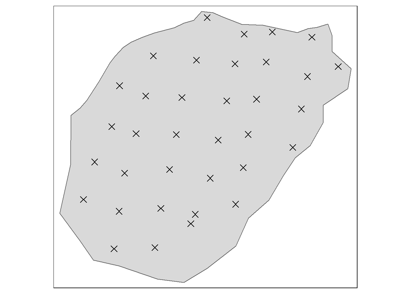
Figure 7.10: Test site Kinn1.
This is a nice example data set. I notice however, there are few points near the edges.
Getting the rough volume
SHP_kinn1$myArea <- sf::st_area(SHP_kinn1)
SHP_kinn1$myArea
#> 13541.53 [m^2]
Mean depth
mean(depths_kinn1_spatial$Dybde, na.rm = T)
#> [1] 244.1429
The depths are in cm. Converting to m.
depths_kinn1_spatial$Dybde <- depths_kinn1_spatial$Dybde/100Number of depth measurements
nrow(depths_kinn1_spatial)
#> [1] 35
Point density (100 m-2)
nrow(depths_kinn1_spatial)/(SHP_kinn1$myArea) * 100
#> 0.2584641 [1/m^2]
Finding optimum power
ccalc_optimumPower(peatDepths = depths_kinn1_spatial,
peatlandDelimination = SHP_kinn1, title = "Kinn1")
#>
|
| | 0%
|
|= | 3%
|
|=== | 6%
|
|==== | 9%
|
|====== | 12%
|
|======= | 15%
|
|========= | 18%
|
|========== | 21%
|
|============ | 24%
|
|============= | 26%
|
|=============== | 29%
|
|================ | 32%
|
|================== | 35%
|
|=================== | 38%
|
|===================== | 41%
|
|====================== | 44%
|
|======================== | 47%
|
|========================= | 50%
|
|========================== | 53%
|
|============================ | 56%
|
|============================= | 59%
|
|=============================== | 62%
|
|================================ | 65%
|
|================================== | 68%
|
|=================================== | 71%
|
|===================================== | 74%
|
|====================================== | 76%
|
|======================================== | 79%
|
|========================================= | 82%
|
|=========================================== | 85%
|
|============================================ | 88%
|
|============================================== | 91%
|
|=============================================== | 94%
|
|================================================= | 97%
|
|==================================================| 100%
#> [inverse distance weighted interpolation]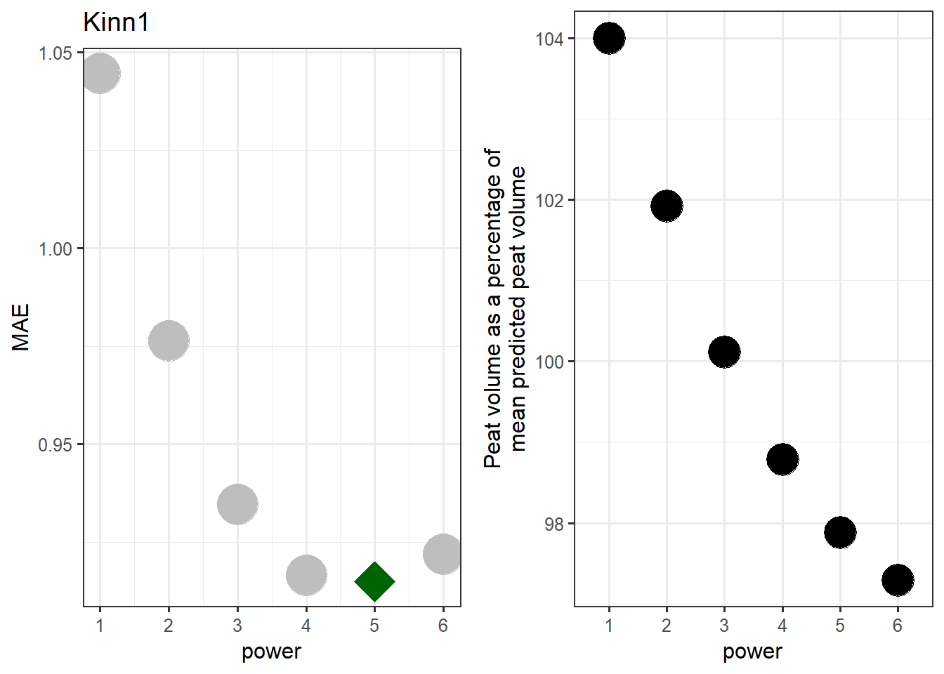
Figure 7.11: Finding the best power setting for the Kinn1 test site.
The optimal power is 5.
Create a raster grid for the predictions
IDW_kinn1_5 <- gstat::idw(Dybde ~ 1, depths_kinn1_spatial,
    newdata = grid_kinn1_stars_crop, nmax = nmax, idp = 5)
#> [inverse distance weighted interpolation]
Max peat depth
max(depths_kinn1_spatial$Dybde)
#> [1] 4.7
myBreaks <- seq(0, 5, 1)
myPos <- c("right", "bottom")

tm_shape(IDW_kinn1_5) + tm_raster(col = "var1.pred",
    palette = "-viridis", title = "Power = 5\nInterpolated peat\ndepth (m)",
    breaks = myBreaks) + tm_compass(type = "8star",
    position = myPos, size = 2) + tm_scale_bar(position = myPos,
    width = 0.3) + tm_shape(depths_kinn1_spatial) +
    tm_symbols(shape = 4, col = "black", size = 0.5) +
    tm_layout(legend.outside = T)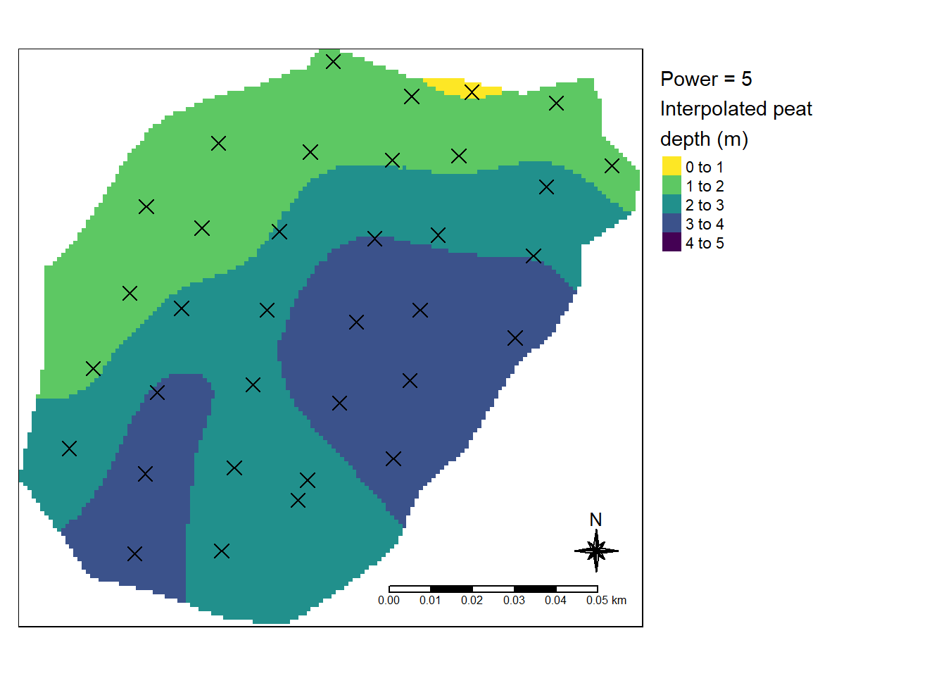
Figure 7.12: Best model for test site Kinn1
Predicted peat volume
(vol_temp <- sum(IDW_kinn1_5$var1.pred, na.rm = T))
#> [1] 33530.09
Carbon stocks
ccalc_cStocks(volume = vol_temp, peatData = df)
#>        5%       50%       95%      mean        sd
#> 1307.8128 1520.3924 1769.1223 1525.8894  133.4278
7.4 Kinn2
SHP_kinn2 <- sf::st_read("Data/Kinn/maroy_avgrensing.shp")
#> Reading layer `maroy_avgrensing' from data source
#>   `C:\Users\anders.kolstad\Github\carbonCalculator\Data\Kinn\maroy_avgrensing.shp'
#>   using driver `ESRI Shapefile'
#> Simple feature collection with 1 feature and 27 fields
#> Geometry type: POLYGON
#> Dimension:     XY
#> Bounding box:  xmin: 5.102353 ymin: 61.50691 xmax: 5.107625 ymax: 61.50866
#> Geodetic CRS:  WGS 84
depths_kinn2 <- read_delim("Data/Kinn/data_maroy_torvdybder.csv",
    delim = ";", escape_double = FALSE, locale = locale(encoding = "ISO-8859-1"),
    trim_ws = TRUE)
As before, the depths have no coordinates.
depths_kinn2_spatial <- sf::st_read("Data/Kinn/maroy_punkter.shp")
#> Reading layer `maroy_punkter' from data source
#>   `C:\Users\anders.kolstad\Github\carbonCalculator\Data\Kinn\maroy_punkter.shp'
#>   using driver `ESRI Shapefile'
#> Simple feature collection with 78 features and 24 fields
#> Geometry type: POINT
#> Dimension:     XYZ
#> Bounding box:  xmin: 5.102523 ymin: 61.50698 xmax: 5.10742 ymax: 61.5086
#> z_range:       zmin: 8.484 zmax: 17.732
#> Geodetic CRS:  WGS 84
depths_kinn2_spatial$name <- as.numeric(depths_kinn2_spatial$name)
depths_kinn2_spatial$Dybde <- depths_kinn2$Dybde[match(depths_kinn2_spatial$name,
    depths_kinn2$name)]
rm(depths_kinn2)
Transform to UTF33
depths_kinn2_spatial <- sf::st_transform(depths_kinn2_spatial,
    25833)
SHP_kinn2 <- sf::st_transform(SHP_kinn2, 25833)
tm_shape(SHP_kinn2) + tm_polygons() + tm_shape(depths_kinn2_spatial) +
    tm_symbols(col = "black", size = 0.5, shape = 4)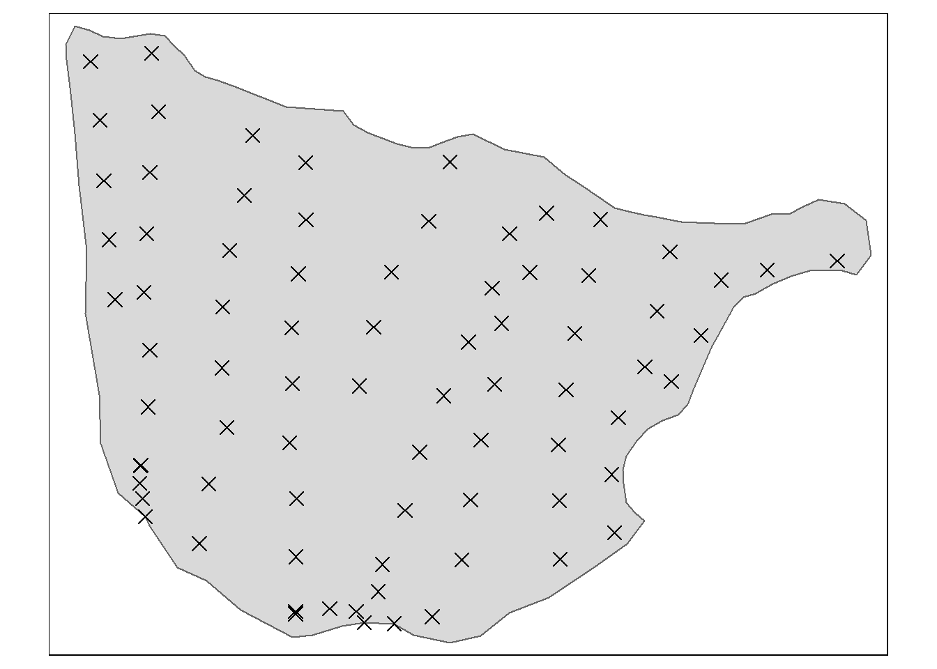
Figure 7.13: Test site Kinn2.
The mean depth
summary(depths_kinn2_spatial$Dybde, na.rm = T)
#>    Min. 1st Qu.  Median    Mean 3rd Qu.    Max.
#>    0.00   41.25   71.00   90.26  130.25  282.00
Converting from cm to m
depths_kinn2_spatial$Dybde <- depths_kinn2_spatial$Dybde/100Calculate area:
SHP_kinn2$myArea <- st_area(SHP_kinn2)Number of peat depth measurements:
nrow(depths_kinn2_spatial)
#> [1] 78
Density of points (100 m-2)
nrow(depths_kinn2_spatial)/SHP_kinn2$myArea * 100
#> 0.2346467 [1/m^2]
Find optimal power
ccalc_optimumPower(peatDepths = depths_kinn2_spatial,
peatlandDelimination = SHP_kinn2, title = "Kinn2")
#>
|
| | 0%
|
|= | 1%
|
|= | 3%
|
|== | 4%
|
|=== | 5%
|
|=== | 6%
|
|==== | 8%
|
|===== | 9%
|
|===== | 10%
|
|====== | 12%
|
|====== | 13%
|
|======= | 14%
|
|======== | 16%
|
|======== | 17%
|
|========= | 18%
|
|========== | 19%
|
|========== | 21%
|
|=========== | 22%
|
|============ | 23%
|
|============ | 25%
|
|============= | 26%
|
|============== | 27%
|
|============== | 29%
|
|=============== | 30%
|
|================ | 31%
|
|================ | 32%
|
|================= | 34%
|
|================== | 35%
|
|================== | 36%
|
|=================== | 38%
|
|=================== | 39%
|
|==================== | 40%
|
|===================== | 42%
|
|===================== | 43%
|
|====================== | 44%
|
|======================= | 45%
|
|======================= | 47%
|
|======================== | 48%
|
|========================= | 49%
|
|========================= | 51%
|
|========================== | 52%
|
|=========================== | 53%
|
|=========================== | 55%
|
|============================ | 56%
|
|============================= | 57%
|
|============================= | 58%
|
|============================== | 60%
|
|=============================== | 61%
|
|=============================== | 62%
|
|================================ | 64%
|
|================================ | 65%
|
|================================= | 66%
|
|================================== | 68%
|
|================================== | 69%
|
|=================================== | 70%
|
|==================================== | 71%
|
|==================================== | 73%
|
|===================================== | 74%
|
|====================================== | 75%
|
|====================================== | 77%
|
|======================================= | 78%
|
|======================================== | 79%
|
|======================================== | 81%
|
|========================================= | 82%
|
|========================================== | 83%
|
|========================================== | 84%
|
|=========================================== | 86%
|
|============================================ | 87%
|
|============================================ | 88%
|
|============================================= | 90%
|
|============================================= | 91%
|
|============================================== | 92%
|
|=============================================== | 94%
|
|=============================================== | 95%
|
|================================================ | 96%
|
|================================================= | 97%
|
|================================================= | 99%
|
|==================================================| 100%
#> [inverse distance weighted interpolation]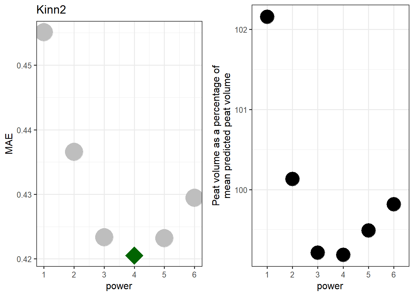
Figure 7.14: Finding the best power setting for the Kinn2 test site.
Power = 4 is best.
Create a raster grid for the predictions
Interpreted peat volume
IDW_kinn2_4 <- gstat::idw(Dybde ~ 1, depths_kinn2_spatial,
    newdata = grid_kinn2_stars_crop, nmax = nmax, idp = 4)
#> [inverse distance weighted interpolation]
myBreaks <- seq(0, 3, 0.5)
myPos <- c("right", "bottom")

tm_shape(IDW_kinn2_4) + tm_raster(col = "var1.pred",
    palette = "-viridis", title = "Power = 4\nInterpolated peat\ndepth (m)",
    breaks = myBreaks) + tm_compass(type = "8star",
    position = myPos, size = 2) + tm_scale_bar(position = myPos,
    width = 0.3) + tm_shape(depths_kinn2_spatial) +
    tm_symbols(shape = 4, col = "black", size = 0.5) +
    tm_layout(legend.outside = T)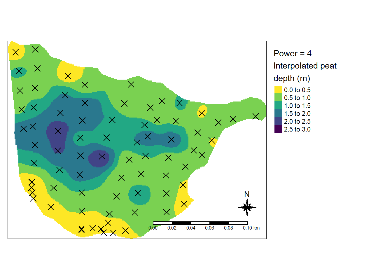
Figure 7.15: Best model for test site Kinn2
And the volume is
(vol_temp <- sum(IDW_kinn2_4$var1.pred, na.rm = T))
#> [1] 33037.11
And the C stock
ccalc_cStocks(volume = vol_temp, peatData = df)
#>       5%      50%      95%     mean       sd
#> 1270.884 1500.529 1710.524 1497.393  134.179