4 Optimise sampling intensity
Now I want to resample and reduce the dataset, but try to keep the original sampling design. For the Geilo dataset I want to limit this part of the analyses to only consider one polygon. It is obvious that a peat depth measurement from a neighboring mire cannot replace data collection on the actual mire.
4.1 Subset Geilo data
# select a single mire polygon
SHP_geilo_biggest <- SHP_geilo[which.max(SHP_geilo$AREAL),
    ]

# drop the depth measurements from the other
# polygons
depths_geilo_biggest <- sf::st_intersection(depths_geilo,
    SHP_geilo_biggest)

# Crop the raster grid
grid_Geilo_stars_crop_biggest <- sf::st_crop(grid_Geilo_stars,
    SHP_geilo_biggest)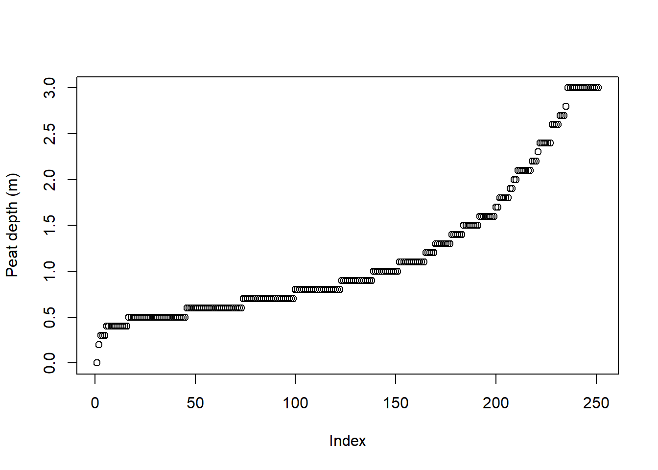
Figure 4.1: Peat depth measurements for the biggest of the Geilo mires.
Looking at the depth measurements in Fig. 4.1, we are reminded that the data contains zeros (measurements taken near the edge) and are truncated above 3 (because that was the length of the peat depth probe).
tm_shape(SHP_geilo_biggest) + tm_polygons() + tm_shape(depths_geilo_biggest) +
    tm_symbols(col = "black", shape = 4)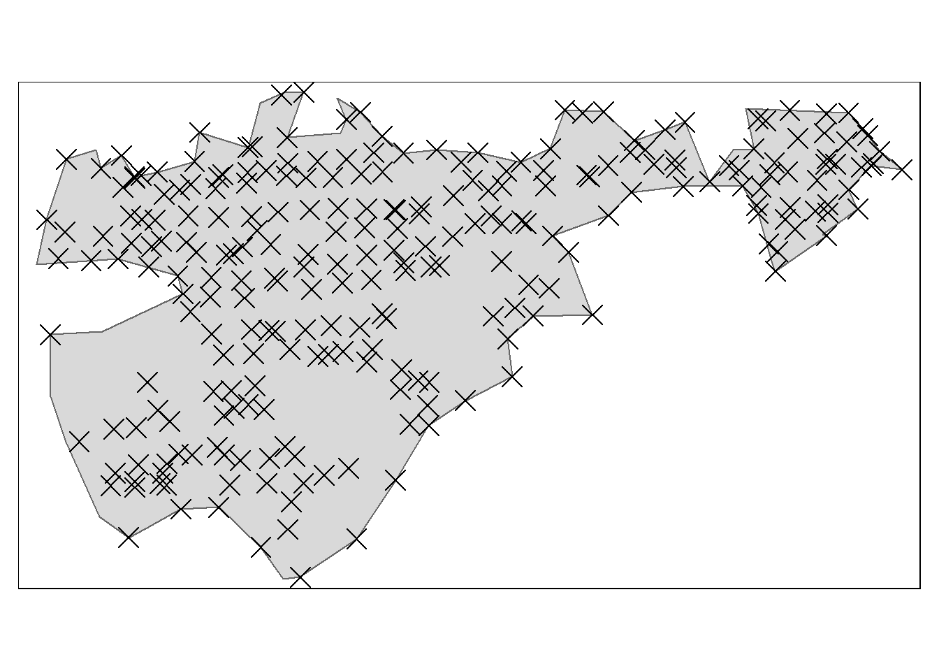
Figure 4.2: One mire polygon from the Geilo test site used in the assessment of minimum sampling.
4.2 Repeat the best IDW
Here I simply recalculate the best models, as described in the previous chapter
IDW_tydal_4 <- gstat::idw(formula = Dybde ~ 1, locations = depths_tydal,
    newdata = grid_Tydal_stars_crop, idp = 4, nmax = nmax)
#> [inverse distance weighted interpolation]

IDW_geilo_3 <- gstat::idw(formula = Dybde ~ 1, locations = depths_geilo_biggest,
    newdata = grid_Geilo_stars_crop_biggest, idp = 3,
    nmax = nmax)
#> [inverse distance weighted interpolation]
4.3 Reduce N
- by gradually removing the closest point.
First we need to set up some temporary files for the for-loop.
distMatrix_tydal <- sf::st_distance(depths_tydal)
distMatrix_tydal <- units::drop_units(distMatrix_tydal)
distMatrix_tydal[distMatrix_tydal == 0] <- NA
distMin_tydal <- matrixStats::rowMins(distMatrix_tydal,
    na.rm = T)

distMatrix_geilo <- sf::st_distance(depths_geilo_biggest)
distMatrix_geilo <- units::drop_units(distMatrix_geilo)
distMatrix_geilo[distMatrix_geilo == 0] <- NA
distMin_geilo <- matrixStats::rowMins(distMatrix_geilo,
    na.rm = T)
Create temporary working files
distMin_tydal_temp <- distMin_tydal
depths_tydal_temp <- depths_tydal

distMin_geilo_temp <- distMin_geilo
depths_geilo_temp <- depths_geilo_biggest
Get the summed volume
est_tydal <- sum(IDW_tydal_4$var1.pred, na.rm = T)
est_geilo <- sum(IDW_geilo_3$var1.pred, na.rm = T)
Get the median, mean and skewness of the distances to the closest neighbor
medianDist_tydal <- median(distMin_tydal)
meanDist_tydal <- mean(distMin_tydal)
skewDist_tydal <- e1071::skewness(distMin_tydal)

medianDist_geilo <- median(distMin_geilo)
meanDist_geilo <- mean(distMin_geilo)
skewDist_geilo <- e1071::skewness(distMin_geilo)
Get the MAE
MAE_tydal_allData <- krige.cv(Dybde ~ 1, depths_tydal,
set = list(idp = 4), nmax = nmax)
#>
|
| | 0%
|
| | 1%
|
|= | 2%
|
|= | 3%
|
|== | 4%
|
|== | 5%
|
|=== | 6%
|
|=== | 7%
|
|==== | 8%
|
|==== | 9%
|
|===== | 10%
|
|===== | 11%
|
|====== | 12%
|
|====== | 13%
|
|======= | 14%
|
|======= | 15%
|
|======== | 16%
|
|======== | 17%
|
|========= | 17%
|
|========= | 18%
|
|========== | 19%
|
|========== | 20%
|
|=========== | 21%
|
|=========== | 22%
|
|============ | 23%
|
|============ | 24%
|
|============= | 25%
|
|============= | 26%
|
|============== | 27%
|
|============== | 28%
|
|=============== | 29%
|
|=============== | 30%
|
|================ | 31%
|
|================ | 32%
|
|================= | 33%
|
|================= | 34%
|
|================= | 35%
|
|================== | 36%
|
|================== | 37%
|
|=================== | 38%
|
|=================== | 39%
|
|==================== | 40%
|
|==================== | 41%
|
|===================== | 42%
|
|===================== | 43%
|
|====================== | 44%
|
|====================== | 45%
|
|======================= | 46%
|
|======================= | 47%
|
|======================== | 48%
|
|======================== | 49%
|
|========================= | 50%
|
|========================== | 51%
|
|========================== | 52%
|
|=========================== | 53%
|
|=========================== | 54%
|
|============================ | 55%
|
|============================ | 56%
|
|============================= | 57%
|
|============================= | 58%
|
|============================== | 59%
|
|============================== | 60%
|
|=============================== | 61%
|
|=============================== | 62%
|
|================================ | 63%
|
|================================ | 64%
|
|================================= | 65%
|
|================================= | 66%
|
|================================= | 67%
|
|================================== | 68%
|
|================================== | 69%
|
|=================================== | 70%
|
|=================================== | 71%
|
|==================================== | 72%
|
|==================================== | 73%
|
|===================================== | 74%
|
|===================================== | 75%
|
|====================================== | 76%
|
|====================================== | 77%
|
|======================================= | 78%
|
|======================================= | 79%
|
|======================================== | 80%
|
|======================================== | 81%
|
|========================================= | 82%
|
|========================================= | 83%
|
|========================================== | 83%
|
|========================================== | 84%
|
|=========================================== | 85%
|
|=========================================== | 86%
|
|============================================ | 87%
|
|============================================ | 88%
|
|============================================= | 89%
|
|============================================= | 90%
|
|============================================== | 91%
|
|============================================== | 92%
|
|=============================================== | 93%
|
|=============================================== | 94%
|
|================================================ | 95%
|
|================================================ | 96%
|
|================================================= | 97%
|
|================================================= | 98%
|
|==================================================| 99%
|
|==================================================| 100%
MAE_tydal_allData <- mean(abs(MAE_tydal_allData$residual))
MAE_geilo_allData <- krige.cv(Dybde ~ 1, depths_geilo_biggest,
set = list(idp = 2), nmax = nmax)
#>
|
| | 0%
|
| | 1%
|
|= | 1%
|
|= | 2%
|
|= | 3%
|
|== | 3%
|
|== | 4%
|
|== | 5%
|
|=== | 5%
|
|=== | 6%
|
|=== | 7%
|
|==== | 7%
|
|==== | 8%
|
|==== | 9%
|
|===== | 9%
|
|===== | 10%
|
|===== | 11%
|
|====== | 11%
|
|====== | 12%
|
|====== | 13%
|
|======= | 13%
|
|======= | 14%
|
|======= | 15%
|
|======== | 15%
|
|======== | 16%
|
|======== | 17%
|
|========= | 17%
|
|========= | 18%
|
|========= | 19%
|
|========== | 19%
|
|========== | 20%
|
|========== | 21%
|
|=========== | 21%
|
|=========== | 22%
|
|=========== | 23%
|
|============ | 23%
|
|============ | 24%
|
|============ | 25%
|
|============= | 25%
|
|============= | 26%
|
|============= | 27%
|
|============== | 27%
|
|============== | 28%
|
|============== | 29%
|
|=============== | 29%
|
|=============== | 30%
|
|=============== | 31%
|
|================ | 31%
|
|================ | 32%
|
|================ | 33%
|
|================= | 33%
|
|================= | 34%
|
|================= | 35%
|
|================== | 35%
|
|================== | 36%
|
|================== | 37%
|
|=================== | 37%
|
|=================== | 38%
|
|=================== | 39%
|
|==================== | 39%
|
|==================== | 40%
|
|==================== | 41%
|
|===================== | 41%
|
|===================== | 42%
|
|===================== | 43%
|
|====================== | 43%
|
|====================== | 44%
|
|====================== | 45%
|
|======================= | 45%
|
|======================= | 46%
|
|======================= | 47%
|
|======================== | 47%
|
|======================== | 48%
|
|======================== | 49%
|
|========================= | 49%
|
|========================= | 50%
|
|========================= | 51%
|
|========================== | 51%
|
|========================== | 52%
|
|========================== | 53%
|
|=========================== | 53%
|
|=========================== | 54%
|
|=========================== | 55%
|
|============================ | 55%
|
|============================ | 56%
|
|============================ | 57%
|
|============================= | 57%
|
|============================= | 58%
|
|============================= | 59%
|
|============================== | 59%
|
|============================== | 60%
|
|============================== | 61%
|
|=============================== | 61%
|
|=============================== | 62%
|
|=============================== | 63%
|
|================================ | 63%
|
|================================ | 64%
|
|================================ | 65%
|
|================================= | 65%
|
|================================= | 66%
|
|================================= | 67%
|
|================================== | 67%
|
|================================== | 68%
|
|================================== | 69%
|
|=================================== | 69%
|
|=================================== | 70%
|
|=================================== | 71%
|
|==================================== | 71%
|
|==================================== | 72%
|
|==================================== | 73%
|
|===================================== | 73%
|
|===================================== | 74%
|
|===================================== | 75%
|
|====================================== | 75%
|
|====================================== | 76%
|
|====================================== | 77%
|
|======================================= | 77%
|
|======================================= | 78%
|
|======================================= | 79%
|
|======================================== | 79%
|
|======================================== | 80%
|
|======================================== | 81%
|
|========================================= | 81%
|
|========================================= | 82%
|
|========================================= | 83%
|
|========================================== | 83%
|
|========================================== | 84%
|
|========================================== | 85%
|
|=========================================== | 85%
|
|=========================================== | 86%
|
|=========================================== | 87%
|
|============================================ | 87%
|
|============================================ | 88%
|
|============================================ | 89%
|
|============================================= | 89%
|
|============================================= | 90%
|
|============================================= | 91%
|
|============================================== | 91%
|
|============================================== | 92%
|
|============================================== | 93%
|
|=============================================== | 93%
|
|=============================================== | 94%
|
|=============================================== | 95%
|
|================================================ | 95%
|
|================================================ | 96%
|
|================================================ | 97%
|
|================================================= | 97%
|
|================================================= | 98%
|
|================================================= | 99%
|
|==================================================| 99%
|
|==================================================| 100%
MAE_geilo_allData <- mean(abs(MAE_geilo_allData$residual))Put it into a dataframe
summaryTable_tydal <- data.frame(medianDist = medianDist_tydal,
    meanDist = meanDist_tydal, skewness = skewDist_tydal,
    n = length(distMin_tydal), estimatedPeatVolume_m3 = est_tydal,
    MAE = MAE_tydal_allData)

summaryTable_geilo <- data.frame(medianDist = medianDist_geilo,
    meanDist = meanDist_geilo, skewness = skewDist_geilo,
    n = length(distMin_geilo), estimatedPeatVolume_m3 = est_geilo,
    MAE = MAE_geilo_allData)
Perform a for-loop to gradually remove points based on how close they are to other points. This will hopefully retain most of the systematic design of the points (avoiding clumping of points).
# I will not bother going lower than ten data
# points
for (i in 1:c(nrow(depths_tydal) - 10)) {

    print(paste("run number = ", i))

    toRemove <- which(distMin_tydal_temp == min(distMin_tydal_temp))[1]
    print(paste("Removing row number ", toRemove))

    # get some stats distance between neighbours
    medianDist <- median(distMin_tydal_temp)
    meanDist <- mean(distMin_tydal_temp)
    skewDist <- e1071::skewness(distMin_tydal_temp)

    depths_tydal_temp <- depths_tydal_temp[-toRemove,
        ]

    # perform interpolation on tempDF
    int <- gstat::idw(Dybde ~ 1, depths_tydal_temp,
        newdata = grid_Tydal_stars_crop, nmax = nmax,
        idp = 4)

    # Export some predictions for checks
    if (i %in% seq(30, 90, 30)) {
        assign(paste0("IDW_tydal_i", i), int)
    }

    est <- sum(int$var1.pred, na.rm = T)

    # get the MAE as well, even though it takes a
    # long time to run
    MAE <- krige.cv(Dybde ~ 1, depths_tydal_temp, set = list(idp = 4),
        nmax = nmax)
    MAE <- mean(abs(MAE$residual))

    # paste into the summary table
    summaryTable_tydal[1 + i, "medianDist"] <- medianDist
    summaryTable_tydal[1 + i, "meanDist"] <- meanDist
    summaryTable_tydal[1 + i, "skewness"] <- skewDist
    summaryTable_tydal[1 + i, "n"] <- length(distMin_tydal_temp) -
        1
    summaryTable_tydal[1 + i, "estimatedPeatVolume_m3"] <- est
    summaryTable_tydal[1 + i, "MAE"] <- MAE

    # prepare dataset for next loop
    euclidDist <- sf::st_distance(depths_tydal_temp)
    euclidDist <- units::drop_units(euclidDist)
    euclidDist[euclidDist == 0] <- NA
    distMin_tydal_temp <- rowMins(euclidDist, na.rm = T)

}
saveRDS(summaryTable_tydal, "Data/Tydal/tydal_cvAnalysisData.rds")

saveRDS(IDW_tydal_i30, "Output/Tydal/IDW_tydal_i30.rds")
saveRDS(IDW_tydal_i60, "Output/Tydal/IDW_tydal_i60.rds")
saveRDS(IDW_tydal_i90, "Output/Tydal/IDW_tydal_i90.rds")
# now doing the same for the Geilo test site
for (i in 1:c(nrow(depths_geilo_biggest) - 10)) {

    print(paste("run number = ", i))

    toRemove <- which(distMin_geilo_temp == min(distMin_geilo_temp))[1]
    print(paste("Removing row number ", toRemove))

    # get some stats distance between neighbours
    medianDist <- median(distMin_geilo_temp)
    meanDist <- mean(distMin_geilo_temp)
    skewDist <- e1071::skewness(distMin_geilo_temp)

    depths_geilo_temp <- depths_geilo_temp[-toRemove,
        ]

    # perform interpolation on tempDF
    int <- gstat::idw(Dybde ~ 1, depths_geilo_temp,
        newdata = grid_Geilo_stars_crop_biggest, nmax = nmax,
        idp = 3)

    # Export some predictions for checks
    if (i %in% seq(40, 240, 50)) {
        assign(paste0("IDW_geilo_i", i), int)
    }

    est <- sum(int$var1.pred, na.rm = T)

    # get the MAE as well, even though it takes a
    # long time to run
    MAE <- krige.cv(Dybde ~ 1, depths_geilo_temp, set = list(idp = 3),
        nmax = nmax)
    MAE <- mean(abs(MAE$residual))

    # paste into the summary table
    summaryTable_geilo[1 + i, "medianDist"] <- medianDist
    summaryTable_geilo[1 + i, "meanDist"] <- meanDist
    summaryTable_geilo[1 + i, "skewness"] <- skewDist
    summaryTable_geilo[1 + i, "n"] <- length(distMin_geilo_temp) -
        1
    summaryTable_geilo[1 + i, "estimatedPeatVolume_m3"] <- est
    summaryTable_geilo[1 + i, "MAE"] <- MAE

    # prepare dataset for next loop
    euclidDist <- sf::st_distance(depths_geilo_temp)
    euclidDist <- units::drop_units(euclidDist)
    euclidDist[euclidDist == 0] <- NA
    distMin_geilo_temp <- rowMins(euclidDist, na.rm = T)

}
saveRDS(summaryTable_geilo, "Data/Geilo/geilo_cvAnalysisData.rds")

saveRDS(IDW_geilo_i40, "Output/Geilo/IDW_geilo_i40.rds")
saveRDS(IDW_geilo_i90, "Output/Geilo/IDW_geilo_i90.rds")
saveRDS(IDW_geilo_i140, "Output/Geilo/IDW_geilo_i140.rds")
saveRDS(IDW_geilo_i190, "Output/Geilo/IDW_geilo_i190.rds")
saveRDS(IDW_geilo_i240, "Output/Geilo/IDW_geilo_i240.rds")
Import the data back in
summaryTable_tydal <- readRDS("Data/Tydal/tydal_cvAnalysisData.rds")
summaryTable_geilo <- readRDS("Data/Geilo/geilo_cvAnalysisData.rds")
A code block just for getting the reduced datasets
distMin_tydal_temp <- distMin_tydal
depths_tydal_temp <- depths_tydal

for (i in 1:c(nrow(depths_tydal) - 10)) {

    # print(paste('run number = ', i))

    toRemove <- which(distMin_tydal_temp == min(distMin_tydal_temp))[1]
    # print(paste('Removing row number ',
    # toRemove))

    depths_tydal_temp <- depths_tydal_temp[-toRemove,
        ]

    # Export some data set for checks
    if (i %in% seq(30, 90, 10)) {
        assign(paste0("depths_tydal_i", i), depths_tydal_temp)
    }

    # prepare dataset for next loop
    euclidDist <- sf::st_distance(depths_tydal_temp)
    euclidDist <- units::drop_units(euclidDist)
    euclidDist[euclidDist == 0] <- NA
    distMin_tydal_temp <- rowMins(euclidDist, na.rm = T)

}


#### Geilo

distMin_geilo_temp <- distMin_geilo
depths_geilo_temp <- depths_geilo_biggest

for (i in 1:c(nrow(depths_geilo_biggest) - 10)) {

    # print(paste('run number = ', i))

    toRemove <- which(distMin_geilo_temp == min(distMin_geilo_temp))[1]
    # print(paste('Removing row number ',
    # toRemove))

    depths_geilo_temp <- depths_geilo_temp[-toRemove,
        ]

    # Export some data set for checks
    if (i %in% c(1, 50, 100, 200)) {
        assign(paste0("depths_geilo_i", i), depths_geilo_temp)
    }

    # prepare dataset for next loop
    euclidDist <- sf::st_distance(depths_geilo_temp)
    euclidDist <- units::drop_units(euclidDist)
    euclidDist[euclidDist == 0] <- NA
    distMin_geilo_temp <- rowMins(euclidDist, na.rm = T)

}
tmap_arrange(tm_shape(SHP_tydal) + tm_polygons() +
    tm_shape(depths_tydal) + tm_symbols(col = "black",
    shape = 4, size = 0.5) + tm_layout(title = "All data points",
    inner.margins = c(0.1, 0.02, 0.1, 0.02)), tm_shape(SHP_tydal) +
    tm_polygons() + tm_shape(depths_tydal_i30) + tm_symbols(col = "black",
    shape = 4, size = 0.5) + tm_layout(title = "-30 data points",
    inner.margins = c(0.1, 0.02, 0.1, 0.02)), tm_shape(SHP_tydal) +
    tm_polygons() + tm_shape(depths_tydal_i60) + tm_symbols(col = "black",
    shape = 4, size = 0.5) + tm_layout(title = "-60 data points",
    inner.margins = c(0.1, 0.02, 0.1, 0.02)), tm_shape(SHP_tydal) +
    tm_polygons() + tm_shape(depths_tydal_i80) + tm_symbols(col = "black",
    shape = 4, size = 0.5) + tm_layout(title = "-80 data points",
    inner.margins = c(0.1, 0.02, 0.1, 0.02)))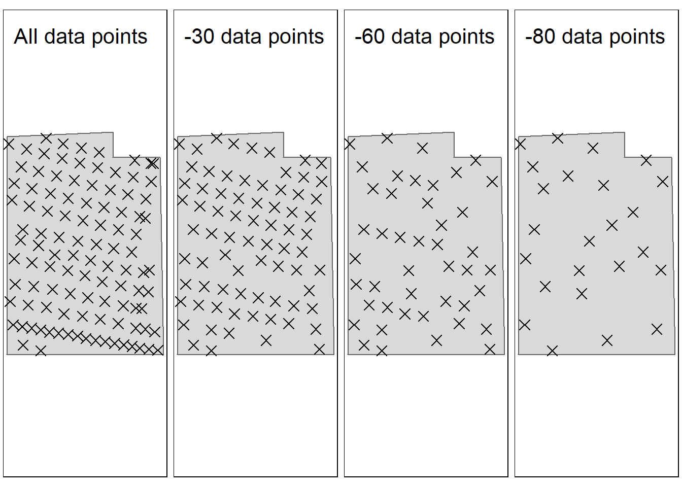
Figure 4.3: Demonstrating the gradual reduction in sampling points. after removing 80 data points, the median distance between the points is 28 meters. Test site: Tydal
tmap_arrange(tm_shape(SHP_geilo_biggest) + tm_polygons() +
    tm_shape(depths_geilo_biggest) + tm_symbols(col = "black",
    shape = 4, size = 0.5) + tm_layout(title = "All data points",
    inner.margins = c(0.1, 0.02, 0.1, 0.02)), tm_shape(SHP_geilo_biggest) +
    tm_polygons() + tm_shape(depths_geilo_i50) + tm_symbols(col = "black",
    shape = 4, size = 0.5) + tm_layout(title = "-50 data points",
    inner.margins = c(0.1, 0.02, 0.1, 0.02)), tm_shape(SHP_geilo_biggest) +
    tm_polygons() + tm_shape(depths_geilo_i100) + tm_symbols(col = "black",
    shape = 4, size = 0.5) + tm_layout(title = "-100 data points",
    inner.margins = c(0.1, 0.02, 0.1, 0.02)), tm_shape(SHP_geilo_biggest) +
    tm_polygons() + tm_shape(depths_geilo_i200) + tm_symbols(col = "black",
    shape = 4, size = 0.5) + tm_layout(title = "-200 data points",
    inner.margins = c(0.1, 0.02, 0.1, 0.02)))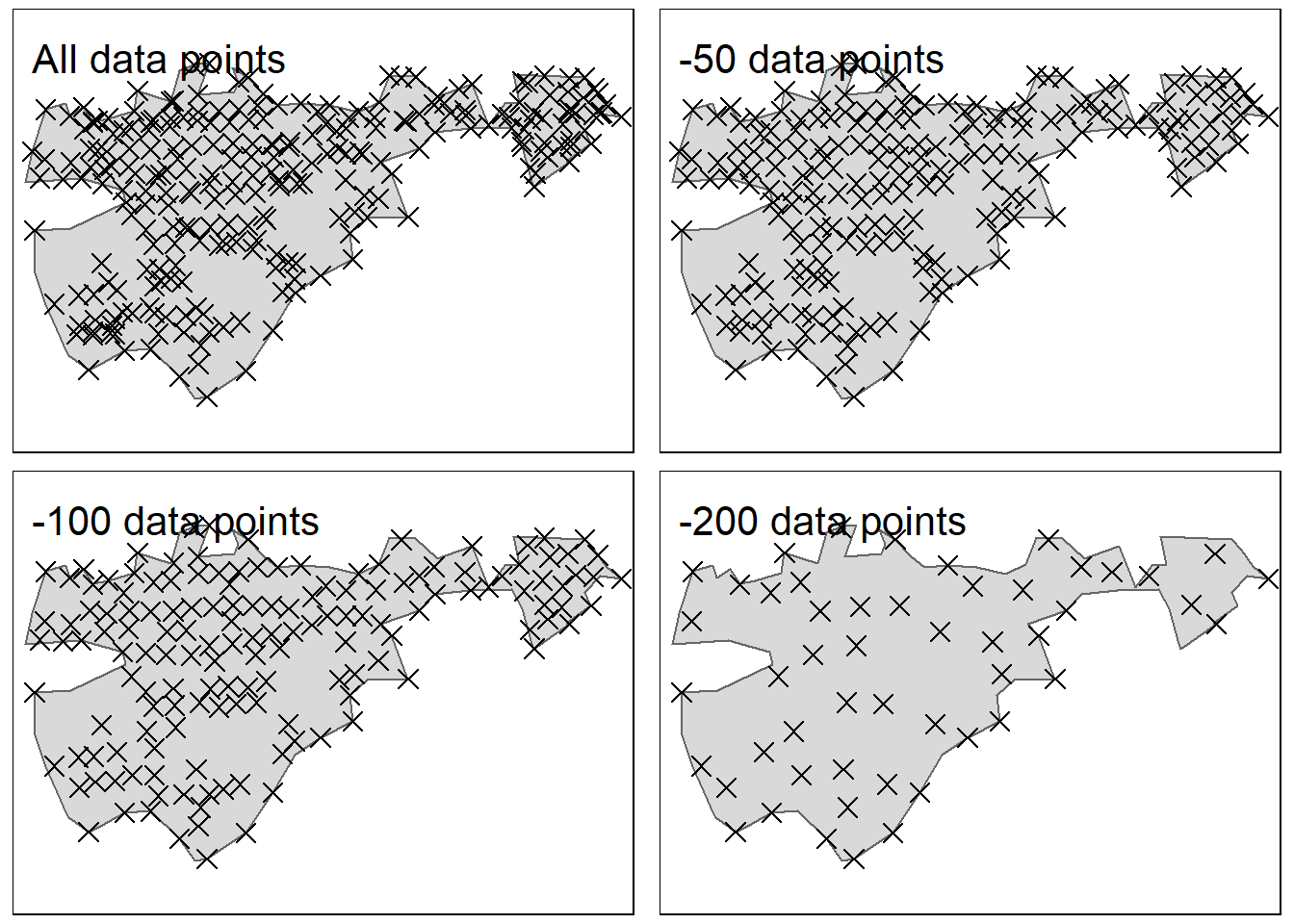
Figure 4.4: Demonstrating the gradual reduction in sampling points. after removinf 200 data poins, the median distance between points is 19 meters. Test site: Geilo
4.4 Explore results
4.4.1 Sampling design
IDW_tydal_i30 <- readRDS("Output/Tydal/IDW_tydal_i30.rds")
IDW_tydal_i60 <- readRDS("Output/Tydal/IDW_tydal_i60.rds")
IDW_tydal_i90 <- readRDS("Output/Tydal/IDW_tydal_i90.rds")
tmap_arrange(tm_shape(IDW_tydal_i30) + tm_raster(col = "var1.pred",
    palette = "-viridis", title = "Interpolated peat\ndepth (m)"),
    tm_shape(IDW_tydal_i60) + tm_raster(col = "var1.pred",
        palette = "-viridis", title = "Interpolated peat\ndepth (m)"),
    tm_shape(IDW_tydal_i90) + tm_raster(col = "var1.pred",
        palette = "-viridis", title = "Interpolated peat\ndepth (m)"))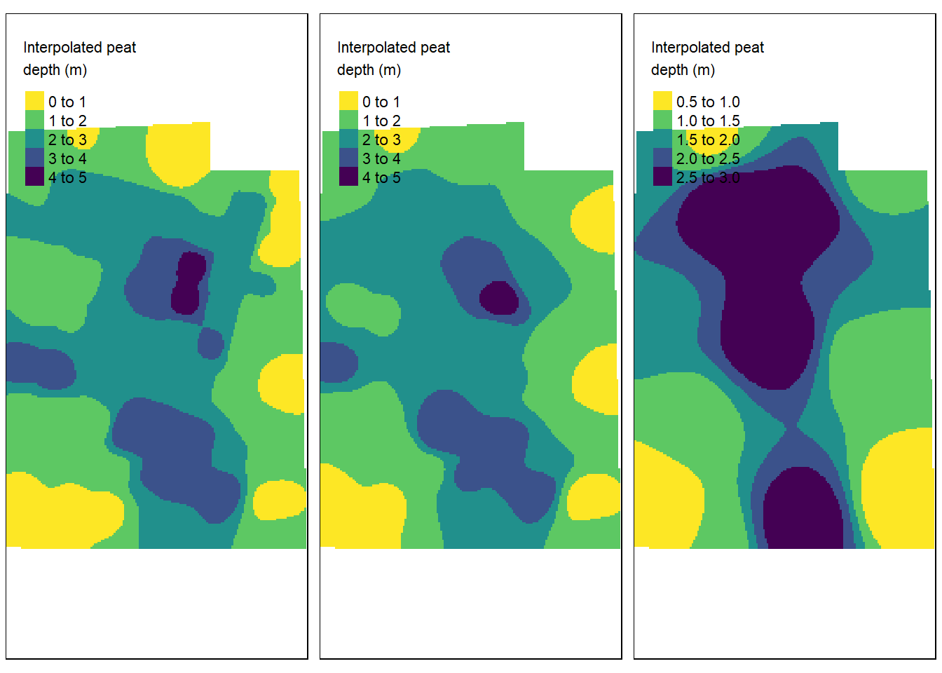
Figure 4.5: IDW with mean distance between data points fromleft to right: 19.4, 20.2 and 40 m. Test site: Tydal
IDW_geilo_i90 <- readRDS("Output/Geilo/IDW_geilo_i90.rds")
IDW_geilo_i140 <- readRDS("Output/Geilo/IDW_geilo_i140.rds")
IDW_geilo_i190 <- readRDS("Output/Geilo/IDW_geilo_i190.rds")
IDW_geilo_i240 <- readRDS("Output/Geilo/IDW_geilo_i240.rds")
tmap_arrange(tm_shape(IDW_geilo_i90) + tm_raster(col = "var1.pred",
    palette = "-viridis", title = "Interpolated peat\ndepth (m)"),
    tm_shape(IDW_geilo_i140) + tm_raster(col = "var1.pred",
        palette = "-viridis", title = "Interpolated peat\ndepth (m)"),
    tm_shape(IDW_geilo_i190) + tm_raster(col = "var1.pred",
        palette = "-viridis", title = "Interpolated peat\ndepth (m)"),
    tm_shape(IDW_geilo_i240) + tm_raster(col = "var1.pred",
        palette = "-viridis", title = "Interpolated peat\ndepth (m)"))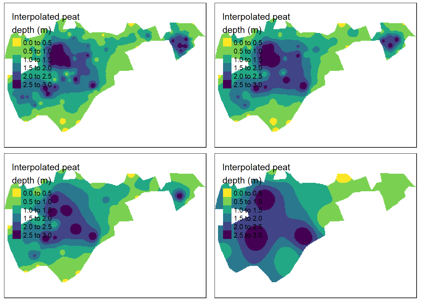
Figure 4.6: IDW with mean distance between data points from left to right, row by row: 9.1, 11.0, 17.3 and 44.5 m. Test site: Geilo
4.4.2 Distance to neighbors
Combine datasets
summaryTable_tydal$site <- "Tydal"
summaryTable_geilo$site <- "Geilo"
summaryTable_twoSites <- rbind(summaryTable_tydal,
    summaryTable_geilo)
ggplot(data = summaryTable_twoSites) + geom_point(aes(x = n,
    y = medianDist)) + geom_point(aes(x = n, y = meanDist),
    pch = 21, fill = "grey") + theme_bw(base_size = 16) +
    ylab("Distance to nearest neighbour (m)") + ylim(0,
    60) + facet_wrap(vars(site), scales = "free_x")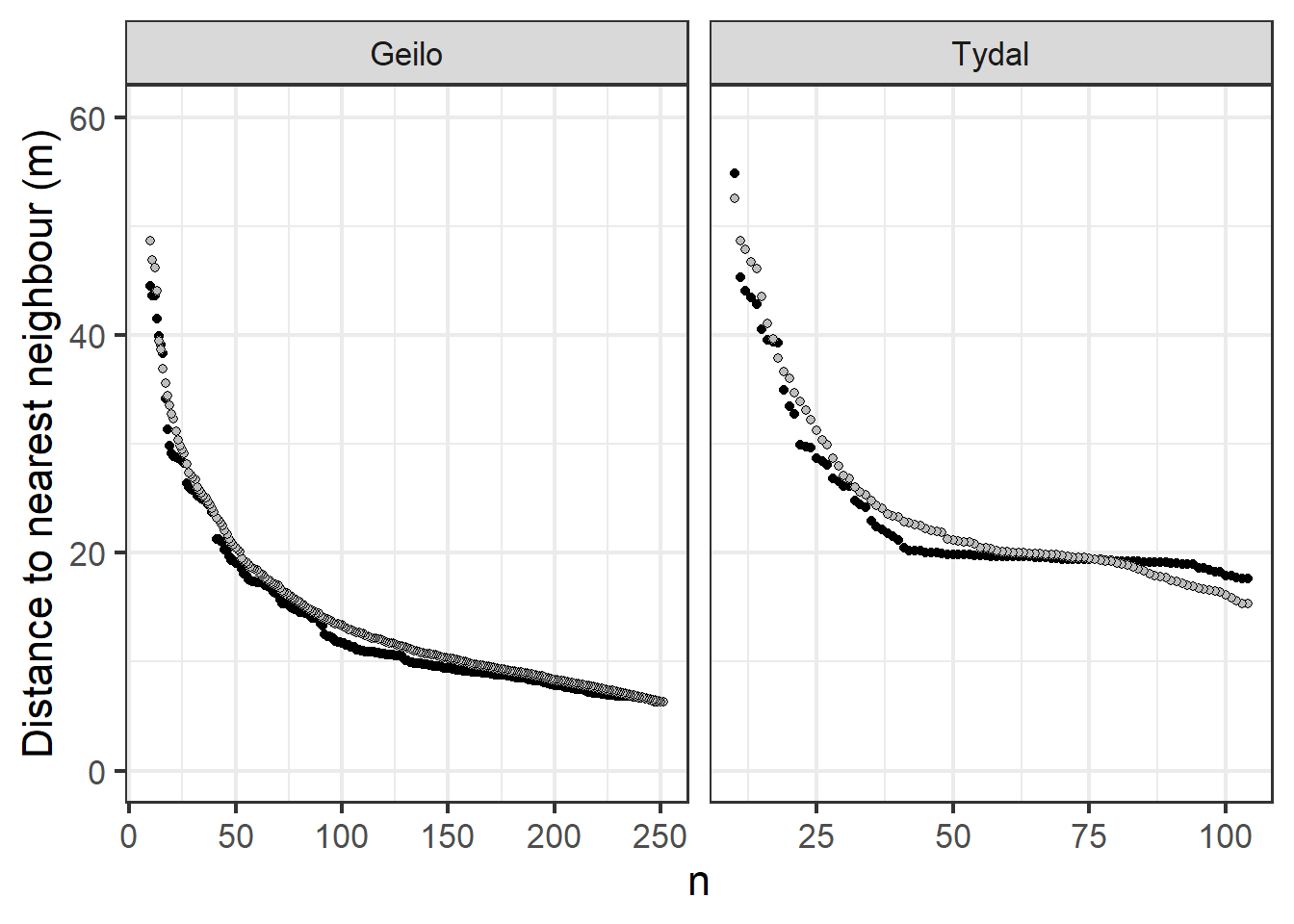
Figure 4.7: Mean (grey) and median (black) distance between peat depth measurements along a gradient of sampling intensity.
This figure tells us that the median (black) and the mean (grey) distance to nearest neighbor are very similar, meaning there is little skew, meaning again that the n reduction process has retained the systematic sampling design.
4.4.3 Skewness
ggplot(data = summaryTable_twoSites) + geom_point(aes(x = n,
    y = skewness), pch = 21, fill = "grey") + theme_bw(base_size = 16) +
    ylab("Skewness") + facet_wrap(vars(site), scales = "free_x")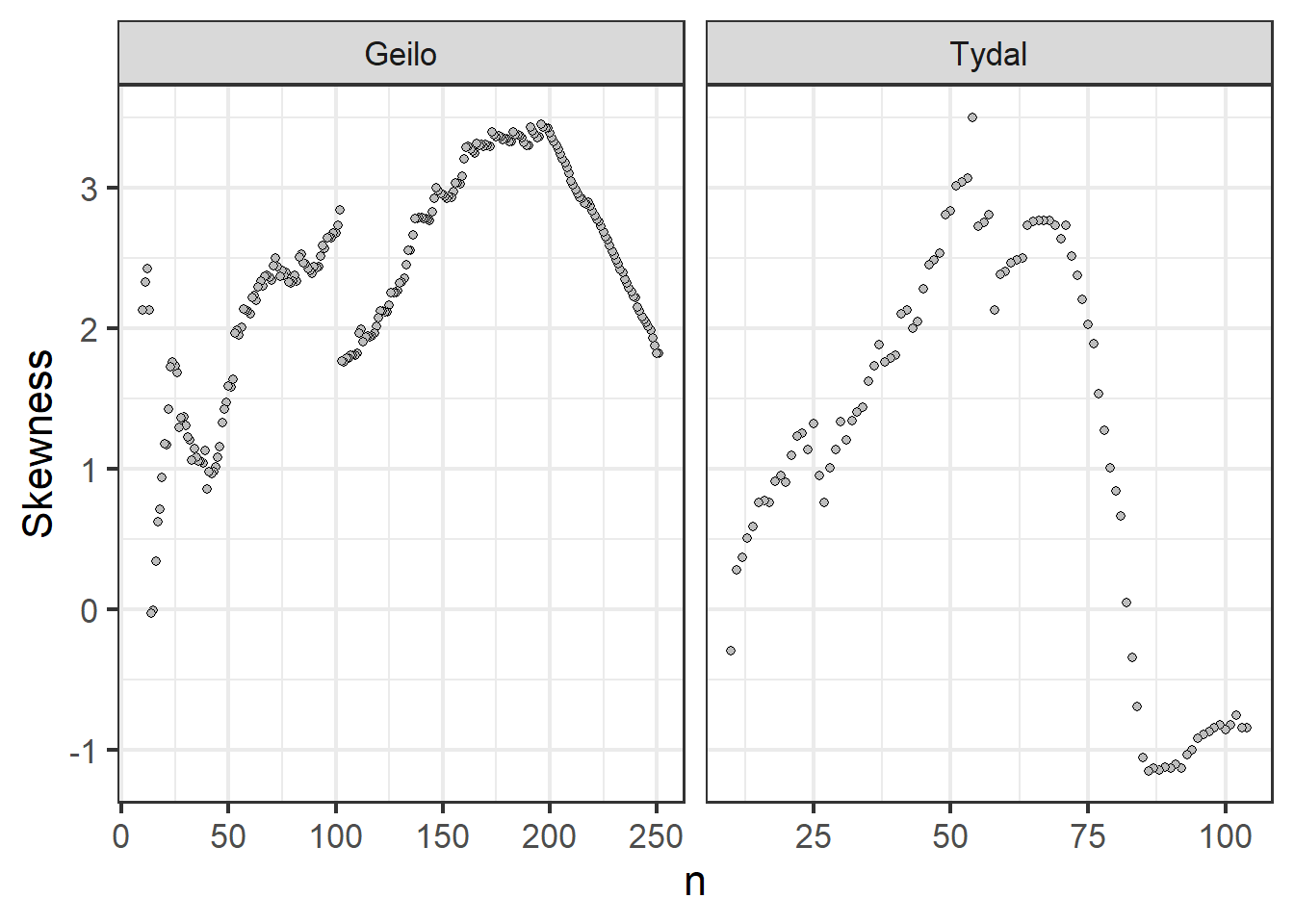
Figure 4.8: Skewness in the distribution of euclidian distances as a response to varying sapling intensity.
Contrary to the above, this figure indicates perhaps that the sampling designs is compromised when I reduce n. It starts out with a negative skew due to some points being very close together. There are then ‘weeded out’ first, and the skew is flipped around to become positive. I will mostly rely on figure 4.3 and 4.4 and say that the reduction in sampling intensity retains the systematic design.
4.4.4 Peat volume estimates
gg_volume <- ggplot(data = summaryTable_twoSites, aes(x = medianDist,
    y = estimatedPeatVolume_m3)) + geom_point(pch = 21,
    fill = "grey", size = 2) + theme_bw(base_size = 16) +
    ylab(expression("Est. peat volume (m"^3 * ")")) +
    xlab("Median distance to nearest neighbour (m)") +
    coord_trans(x = "log2") + facet_wrap(vars(site),
    scales = "free")


ggsave("Output/plot_distanceAgainstVolume.tiff", gg_volume,
    width = 1600, height = 1200, units = "px")
library(svglite)
ggsave("Output/Figure1.svg", gg_volume, width = 7,
    height = 5)

gg_volume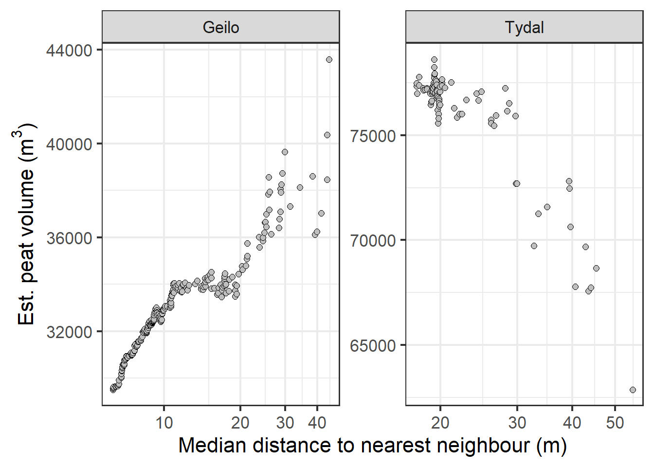
Figure 4.9: Estimated peat volume as a response of the median distance between sampling points.
For Tydal, the estimated peat volume is quite stable up to around 25 meter between sampling points. For Geilo, the estimated volume increases from zero to 10-12 meters, before stabilizing and finally increasing again with distances above 29 meters. The most correct prediction comes with a median distance between 12-20 meters. The original sampling density was biased towards the edges, resulting in a disproportionate large number of samples from shallow areas (Fig. 4.4 ). The IDW does not seem to be able to adequately control for this, and care should be taken to ensure a balanced and systematic sampling design.
4.4.5 CV
In addition to seeing the peat volume estimates becoming biased with increasing distance between sampling points, we also we the variation increasing. Now we will calculate this in terms of the coefficient of variation.
max(summaryTable_tydal$medianDist)
#> [1] 54.87518
max(summaryTable_geilo$medianDist)
#> [1] 44.49275
tydal_cv <- summaryTable_tydal
tydal_cv$group <- ifelse(tydal_cv$medianDist < 10,
    "<10 m", ifelse(tydal_cv$medianDist < 15, "10-15 m",
        ifelse(tydal_cv$medianDist < 20, "15-20 m",
            ifelse(tydal_cv$medianDist < 25, "20-25 m",
                ifelse(tydal_cv$medianDist < 30, "25-30 m",
                  ifelse(tydal_cv$medianDist < 35,
                    "30-35 m", ifelse(tydal_cv$medianDist <
                      40, "35-40 m", "40-55 m")))))))
tydal_cv <- tydal_cv[tydal_cv$medianDist < 100, ]
(tydal_n <- table(tydal_cv$group))
#>
#> 15-20 m 20-25 m 25-30 m 30-35 m 35-40 m 40-55 m
#>      60      13      10       3       3       6
There’s quite few data points in the higher categories. Perhaps too few.
geilo_cv <- summaryTable_geilo
geilo_cv$group <- ifelse(geilo_cv$medianDist < 10,
    "<10 m", ifelse(geilo_cv$medianDist < 15, "10-15 m",
        ifelse(geilo_cv$medianDist < 20, "15-20 m",
            ifelse(geilo_cv$medianDist < 25, "20-25 m",
                ifelse(geilo_cv$medianDist < 30, "25-30 m",
                  ifelse(geilo_cv$medianDist < 35,
                    "30-35 m", ifelse(geilo_cv$medianDist <
                      40, "35-40 m", "40-55 m")))))))
geilo_cv <- geilo_cv[geilo_cv$medianDist < 100, ]
(geilo_n <- table(geilo_cv$group))
#>
#>   <10 m 10-15 m 15-20 m 20-25 m 25-30 m 30-35 m 35-40 m
#>     120      56      29      13      15       2       3
#> 40-55 m
#>       4
CV function
tydal_cv_tbl <- tapply(tydal_cv$estimatedPeatVolume_m3,
    tydal_cv$group, cv)
tydal_cv_tbl <- data.frame(cv = tydal_cv_tbl, label = names(tydal_cv_tbl),
    order = c(3, 4, 5, 6, 7, 8))
tydal_cv_tbl <- tydal_cv_tbl[order(tydal_cv_tbl$order),
    ]
tydal_cv_tbl$n <- tydal_n

geilo_cv_tbl <- tapply(geilo_cv$estimatedPeatVolume_m3,
    geilo_cv$group, cv)
geilo_cv_tbl <- data.frame(cv = geilo_cv_tbl, label = names(geilo_cv_tbl),
    order = c(1, 2, 3, 4, 5, 6, 7, 8))
geilo_cv_tbl <- geilo_cv_tbl[order(geilo_cv_tbl$order),
    ]
geilo_cv_tbl$n <- geilo_n
Join tables
tydal_cv_tbl$site = "Tydal"
geilo_cv_tbl$site = "Geilo"
cvTab <- rbind(tydal_cv_tbl, geilo_cv_tbl)
gg_cv <- ggplot(data = cvTab, aes(x = order, y = cv,
    fill = site, shape = site)) + geom_line(lty = 2) +
    scale_shape_manual(values = c(21, 24)) + geom_point(size = 3,
    stroke = 1.5, position = position_dodge(width = 0.2)) +
    theme_bw(base_size = 16) + scale_x_continuous(breaks = cvTab$order,
    labels = cvTab$label) + theme(axis.text.x = element_text(angle = 90)) +
    xlab("")

ggsave("Output/plot_distanceAgainstCV.tiff", gg_cv,
    width = 1600, height = 1200, units = "px")

gg_cv
Figure 4.10: Coefficient of variation in peat volume estimates as a response to median distance between sampling points
4.5 MAE
gg_mae <- ggplot(data = summaryTable_twoSites, aes(x = medianDist,
    y = MAE)) + geom_point(pch = 21, fill = "grey",
    size = 2) + theme_bw(base_size = 16) + ylab("Mean absolute error (m)") +
    xlab("Median distance to nearest neighbour (m)") +
    coord_trans(x = "log2") + facet_wrap(vars(site),
    scales = "free")


ggsave("Output/plot_distanceAgainstMAE.tiff", gg_mae,
    width = 1600, height = 1200, units = "px")

gg_mae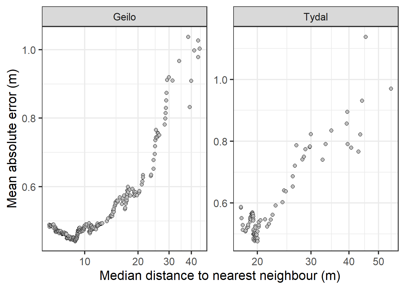
Figure 4.11: MAE in IDW predictions as a response of median distance between sampling points.
This figure I think also supports that sampling distances above about 25 m is a bad idea.