Load packages
library(tidyverse)
library(readxl)
library(DT)
library(ggplot2)
library(kableExtra)library(tidyverse)
library(readxl)
library(DT)
library(ggplot2)
library(kableExtra)The data set is located on GitHub in an xlsx format. The data are split into different tabs based on year.
dat <- read_excel("data/growthData.xlsx",
    sheet = "y2017") |>
  # remove some measurements from October (FALL2).
  # These were measured again in November
  # along with the rest of the quadrats.
  select(-DateFALL2,
         -HeightFALL2,
         -ObserverFALL2) |>
  # adding a variable that keeps track of which tab the data comes from
  add_column(tab_year = 2017) |>
  bind_rows(
    read_excel("data/growthData.xlsx",
    sheet = "y2018") |>
  mutate(DateFALL = as.Date(DateFALL, "%d.%m.%Y"),
         tab_year = 2018)
         ) |>
  bind_rows(
    read_excel("data/growthData.xlsx",
    sheet = "y2019") |>
    mutate(
      DateSUMMER = as.Date(DateSUMMER, "%d/%m/%Y"),
      DateFALL = as.Date(DateFALL, "%d/%m/%y"),
      tab_year = 2019)
  ) |>
  bind_rows(
    read_excel("data/growthData.xlsx",
    sheet = "y2020") |>
    mutate(DateSPRING = as.Date(DateSPRING, "%d/%m/%Y"),
           tab_year = 2020)
  ) |>
  bind_rows(
    read_excel("data/growthData.xlsx",
    sheet = "y2021") |>
      # data had explicit NAs in cells that were read as text:
    mutate(across(starts_with("Height"), as.numeric),
           tab_year = 2021)
  ) |>
  bind_rows(
    read_excel("data/growthData.xlsx",
    sheet = "y2022") |>
    mutate(across(starts_with("Height"), as.numeric),
           Plot_no = as.numeric(Plot_no),
           Pin_no = as.numeric(Pin_no),
           tab_year = 2022)
  )
There are some warnings when actual NAs (text) are converted to real NAs.
Here’s what the data looks like after I just row bind them:
DT::datatable(dat |> slice_sample(n = 10))I need to make this into a long format. There are multiple date and height columns that I want to combine. I will split the spring and fall data (ignoring the summer data) into separate sets, and then combine them again later.
# Spring data
dat_spring <- dat |>
  select(-contains(c("FALL", "SUMMER", "diff"))) |>
  pivot_longer(
    cols = contains("Height"),
    values_to = "Height_cm",
    values_drop_na = T
  ) |>
  separate_wider_delim(name,
    delim = "_",
    names = c("temp", "pinPosition"),
    too_few = "align_start"
  ) |>
  filter(str_detect(temp, "Rejected", negate = T)) |>
  mutate(pinPosition = case_when(
    is.na(pinPosition) ~ "single",
    .default = pinPosition
  )) |>
  select(-temp) |>
  add_column(season = "spring") |>
  rename(date = DateSPRING)

# names(dat) [!names(dat) %in% names(dat_spring) ]
# unique(dat_spring$pinPosition)


dat_fall <- dat |>
  select(-contains(c("SPRING", "SUMMER", "diff"))) |>
  # introduces NA, where NA was originally as text
  mutate(across(starts_with("Height"), as.numeric)) |>
  pivot_longer(
    cols = contains("Height"),
    values_to = "Height_cm",
    values_drop_na = T
  ) |>
  separate_wider_delim(name,
    delim = "_",
    names = c("temp", "pinPosition"),
    too_few = "align_start"
  ) |>
  filter(str_detect(temp, "Rejected", negate = T)) |>
  mutate(pinPosition = case_when(
    is.na(pinPosition) ~ "single",
    .default = pinPosition
  )) |>
  select(-temp) |>
  add_column(season = "fall") |>
  rename(date = DateFALL)

# A check looking into the warnings introduced when turning
# Hieght columns from characters to numeric. All fine.
# ch <- dat |>
#   select(-contains(c("SPRING", "SUMMER", "diff"))) |>
#   drop_na(HeightFALL) |>
#   unite("link", c(ID, DateFALL))
# num <- dat |>
#   select(-contains(c("SPRING", "SUMMER", "diff"))) |>
#   mutate(across(starts_with("Height"), as.numeric)) |>
#   drop_na(HeightFALL) |>
#   unite("link", c(ID, DateFALL))
# ch |>
#   filter(!link %in% num$link) |>
#   View()


# Combining the two
dat_long <- dat_spring |>
  bind_rows(dat_fall) |>
  # merge comments and note columns
  unite("Remarks",
    contains(c("Comment", "Notes")),
    sep = ". ",
    na.rm = TRUE
  ) |>
  # merge observer columns
  unite("Observer",
    contains("Observer"),
    sep = ". ",
    na.rm = TRUE
  ) |>
  mutate(year = year(date))

rm(dat_fall, dat_spring)
The long data is 14641 rows. This is too much to display as an html table on this web site, but here is a random sample of 50 rows just to illustrate.
DT::datatable(dat_long |> slice_sample(n = 50))A closer look at the Treatment variable.
dat_long |>
  count(Treatment)
# A tibble: 10 × 2
Treatment n
<chr> <int>
1 EDGE 492
2 HOLLOW 1642
3 HUMMOCK 762
4 K 1888
5 M 2046
6 R1 1941
7 R2 1917
8 T1 1923
9 T2 1958
10 <NA> 72How can Treatment be NA? Turns out these are all new pins, and all from the fall. I will delete the rows for a different reason below.
Are the dates entered correctly to match the seasons?
dat_long |>
  ggplot() +
  geom_bar(aes(x = month(date)))+
  facet_grid(year(date)~season)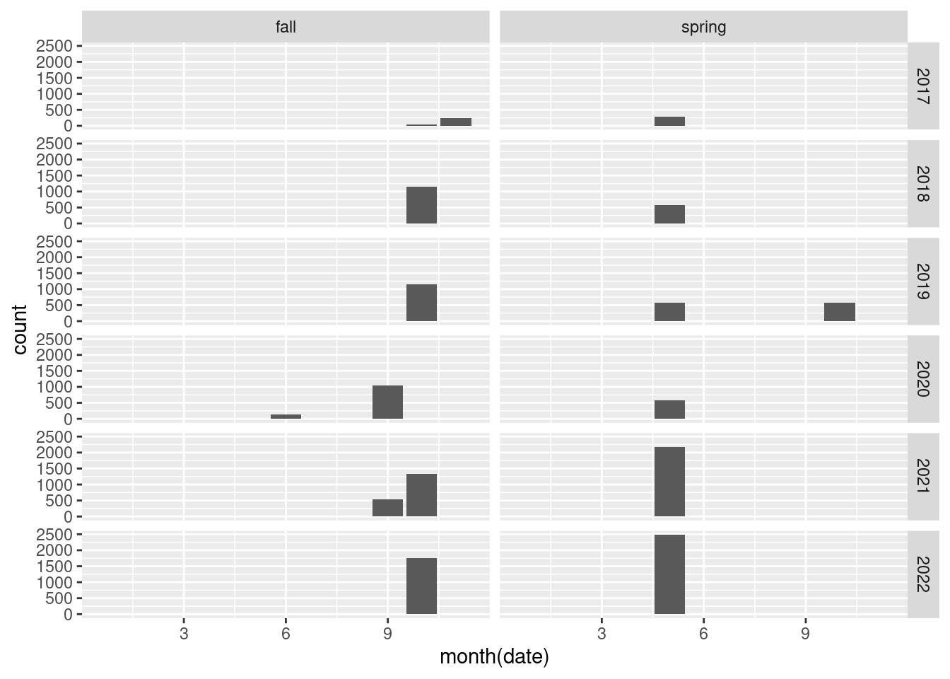
There are some measurements in the fall of 2020 that are wrong. It turns out the month and day have been switched for plots 8 and 9:
dat_long |>
  mutate(year = year(date)) |>
  filter(year == 2020,
         season == "fall") |>
  ggplot() +
  geom_bar(aes(x = date),
           color = "yellow",
           fill = "orange")+
  theme(axis.text.y = element_blank()) +
  facet_grid(Plot_no~.)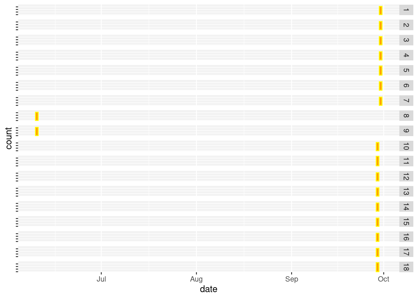
dat_long |>
  filter(Plot_no %in% c(8, 9),
         season == "fall",
         year(date) == 2020) |>
  View()
I will reverse these now.
dat_long <- dat_long |>
  mutate(date = case_when(
    Plot_no %in% c(8,9) & date == date("2020-06-10") ~ date("2020-10-06"),
    .default = date
))dat_long |>
mutate(year = year(date)) |>
filter(year == 2020,
season == "fall") |>
ggplot() +
geom_bar(aes(x = date),
color = "yellow",
fill = "orange")+
theme(axis.text.y = element_blank()) +
facet_grid(Plot_no~.)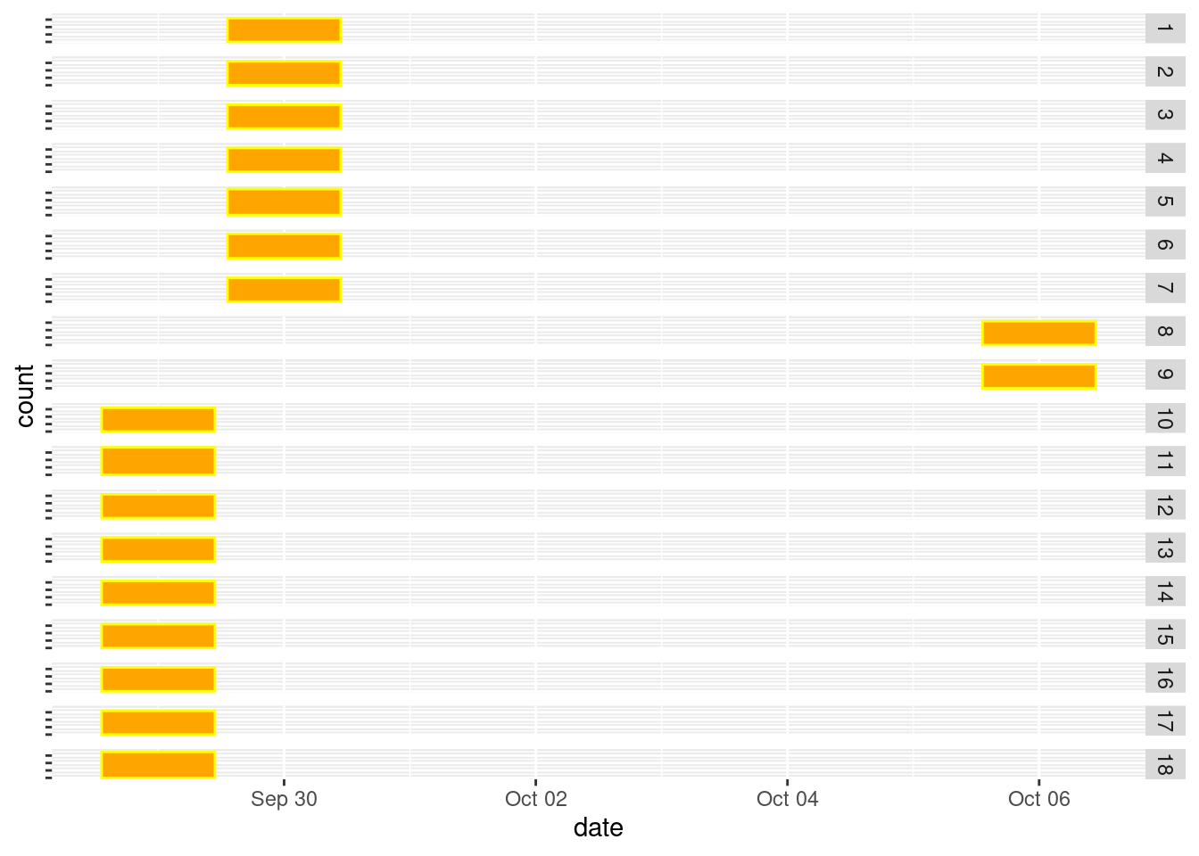
Then there were some errors with the dates in the spring of 2019 Figure 2.1.
dat_long |>
  filter(year == 2019,
         season == "spring") |>
  mutate(month = month(date)) |>
  group_by(date, month) |>
  count()
# A tibble: 2 × 3
# Groups: date, month [2]
date month n
<dttm> <dbl> <int>
1 2019-05-15 00:00:00 5 584
2 2019-10-05 00:00:00 10 576Here I will assume that it is only the month that is wrong. Fixing this now:
dat_long |>
  mutate(date = case_when(
    year == 2019 & date == date("2019-10-05") ~ date("2019-05-10"),
    .default = date
  )) |>
  filter(year == 2019,
         season == "spring") |>
  mutate(month = month(date)) |>
  group_by(date, month) |>
  count()
# A tibble: 2 × 3
# Groups: date, month [2]
date month n
<dttm> <dbl> <int>
1 2019-05-10 00:00:00 5 576
2 2019-05-15 00:00:00 5 584# OK
dat_long <- dat_long |>
mutate(date = case_when(
year == 2019 & date == date("2019-10-05") ~ date("2019-05-10"),
.default = date
))dat_long |>
ggplot() +
geom_bar(aes(
x = factor(year(date)),
fill = season)) +
labs(x = "Year")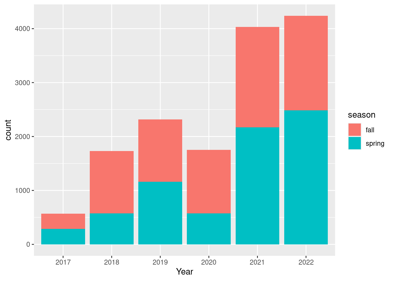
I wonder why there are so relatively few observation in spring 2020.
options(knitr.kable.NA = '')

dat_long |>
  mutate(tab_year = paste0("tab_year", tab_year)) |>
  group_by(tab_year, year) |>
  count() |>
  spread(year, n) |>
  knitr::kable() |>
kable_paper(full_width = F)| tab_year | 2017 | 2018 | 2019 | 2020 | 2021 | 2022 |
|---|---|---|---|---|---|---|
| tab_year2017 | 570 | |||||
| tab_year2018 | 1729 | |||||
| tab_year2019 | 2316 | |||||
| tab_year2020 | 1752 | 576 | ||||
| tab_year2021 | 4034 | |||||
| tab_year2022 | 3664 |
Turns out some of the 2020 data (those added to the 2020 tab) was give the wrong date.
dat_long |>
  mutate(date = case_when(
    tab_year == 2020 & year == 2022 ~ date - years(2),
    .default = date),
         year = year(date))|>
  mutate(tab_year = paste0("tab_year", tab_year)) |>
  group_by(tab_year, year) |>
  count() |>
  spread(year, n) |>
  knitr::kable() |>
kable_paper(full_width = F)| tab_year | 2017 | 2018 | 2019 | 2020 | 2021 | 2022 |
|---|---|---|---|---|---|---|
| tab_year2017 | 570 | |||||
| tab_year2018 | 1729 | |||||
| tab_year2019 | 2316 | |||||
| tab_year2020 | 2328 | |||||
| tab_year2021 | 4034 | |||||
| tab_year2022 | 3664 |
# OK

dat_long <- dat_long |>
  mutate(date = case_when(
    tab_year == 2020 & year == 2022 ~ date - years(2),
    .default = date),
year = year(date))dat_long |>
ggplot() +
geom_bar(aes(
x = year,
fill = season)) +
labs(x = "Year")
dat_long |>
  group_by(year, season) |>
  count(pinPosition) |>
  spread(pinPosition, n) |>
  kable() |>
kable_paper()| year | season | E1 | E2 | H1 | H2 | single | V1 | V2 | W1 | W2 |
|---|---|---|---|---|---|---|---|---|---|---|
| 2017 | fall | 281 | ||||||||
| 2017 | spring | 289 | ||||||||
| 2018 | fall | 288 | 288 | 289 | 289 | |||||
| 2018 | spring | 287 | 288 | |||||||
| 2019 | fall | 289 | 289 | 289 | 289 | |||||
| 2019 | spring | 290 | 290 | 290 | 290 | |||||
| 2020 | fall | 300 | 288 | 300 | 288 | |||||
| 2020 | spring | 288 | 288 | 288 | 288 | |||||
| 2021 | fall | 467 | 466 | 467 | 466 | |||||
| 2021 | spring | 543 | 541 | 543 | 541 | |||||
| 2022 | fall | 439 | 441 | 437 | 439 | |||||
| 2022 | spring | 478 | 478 | 476 | 476 |
I want to combine E1 with E2, H1 with H2, etc.
In addition, in 2018 I want to combine all pinPositions. In 2018, V (venstre) can be made equivalent W (west) , and H is E.
dat_long |>
  mutate(pinPosition2 = case_match(
    pinPosition,
    c("H1", "H2", "V1", "V2") ~ "single",
    c("E1", "E2") ~ "E",
    c("W1", "W2") ~ "W",
    .default = pinPosition
  )) |>
  count(pinPosition2)
 # OK. This variable can be aggregated across

dat_long <- dat_long |>
  mutate(pinPosition2 = case_match(
    pinPosition,
    c("H1", "H2", "V1", "V2") ~ "single",
    c("E1", "E2") ~ "E",
    c("W1", "W2") ~ "W",
    .default = pinPosition
)) dat_long |>
group_by(year, season) |>
count(pinPosition2) |>
spread(pinPosition2, n) |>
kbl() |>
kable_paper(full_width=F)| year | season | E | single | W |
|---|---|---|---|---|
| 2017 | fall | 281 | ||
| 2017 | spring | 289 | ||
| 2018 | fall | 1154 | ||
| 2018 | spring | 575 | ||
| 2019 | fall | 578 | 578 | |
| 2019 | spring | 580 | 580 | |
| 2020 | fall | 588 | 588 | |
| 2020 | spring | 576 | 576 | |
| 2021 | fall | 933 | 933 | |
| 2021 | spring | 1084 | 1084 | |
| 2022 | fall | 880 | 876 | |
| 2022 | spring | 956 | 952 |
A closer look at the ID variable.
Here’s the time series for a single pin, measured from the west.
dat_long |>
  filter(grepl("^8.14", ID),
         pinPosition == "W2") |>
  arrange(year) |>
  select(ID, Remarks, year, season, Height_cm) |>
  datatable()
It appears the pin was replaced in the fall of 2019. I must assume that what is recorded there is the height of the new pin, and is therefore not compareable to the spring value that same year. The new annotation only last one time, i.e. it is not repeated the next season. In the spring of 2021 the wire seems to have been replaced again, and then again in the fall. In the spring of 2022 it was replaced a forth(?) time, according to the remarks. But this time the ID is unchanged.
Conclusion. I will calculate the growth per season, if and only if the spring and fall height are recorded on the same pin/wire. That means I can remove seasons where the fall measurements are done on new wires. There are also some IDs that have the suffix old. In these cases there should always be one measurement for the same date with the prefix new, meaning I can delete all old measurements from the spring heights.
dat_long |>
  separate_wider_regex(ID,
    c(ID_num = "\\d+.\\d++", text_in_ID = "\\w+"),
    too_few = "align_start",
    cols_remove = F) |>
  count(text_in_ID)
# A tibble: 5 × 2
text_in_ID n
<chr> <int>
1 NØ 2
2 SV 1
3 new 964
4 old 348
5 <NA> 13326I will split the ID column into a numerical ID_num, and a text_in_ID field that contains the suffix, if any (e.g. old or new). In the same go I remove those with direction (NØ or SV) in the ID.
dat_long <- dat_long|>
  separate_wider_regex(ID,
    c(ID_num = "\\d+.\\d++", text_in_ID = "\\w+"),
    too_few = "align_start",
    cols_remove = F) |>
  filter(!text_in_ID %in% c("NØ", "SV"))
Then I remove those that are old in spring. I thought I could also remove those that are new in the fall, but turn out these could be labeled new in spring, and then that label is kept though that season (and reset again in the next season). First, here is a view of the occurrences of old and new IDs.
dat_long <- dat_long |>
  mutate(text_in_ID = case_when(
    is.na(text_in_ID) ~ "-",
    .default = text_in_ID
  ))

dat_long |>
  group_by(year, season) |>
  count(text_in_ID) |>
  spread(text_in_ID, n) |>
  select(-"-") |>
  kbl() |>
kable_paper(full_width = F)| year | season | new | old |
|---|---|---|---|
| 2017 | fall | ||
| 2017 | spring | ||
| 2018 | fall | 36 | |
| 2018 | spring | ||
| 2019 | fall | 60 | 4 |
| 2019 | spring | 8 | 12 |
| 2020 | fall | 48 | 24 |
| 2020 | spring | 48 | |
| 2021 | fall | 400 | 4 |
| 2021 | spring | 412 | 256 |
| 2022 | fall | ||
| 2022 | spring |
I need to remove those that are new in fall and that don’t have any value labeled new in spring (i.e. that they are truly new that fall, and that the label is not simply carried from the spring record). Similarly, I want to remove those that are old in fall, and don’t have any values labeled old in the preceding spring. First I create a link variable for the occurrences that I want to match against.
newInSpring <- dat_long |>
  filter(season == "spring" & text_in_ID == "new") |>
  mutate(link = paste(ID_num, tab_year, pinPosition, sep= "_")) |>
  pull(link)

oldInFall <- dat_long |>
  filter(season == "fall" & text_in_ID == "old") |>
  mutate(link = paste(ID_num, tab_year+1, pinPosition, sep= "_")) |>
  pull(link)
Then I remove some records based on this link variable.
dat_long <- dat_long |>
  mutate(link = paste(ID_num, tab_year, pinPosition, sep= "_")) |>
  filter(
    ifelse(text_in_ID == "new" & !link %in% newInSpring,
      season != "fall",
      TRUE),
    ifelse(text_in_ID == "old" & !link %in% oldInFall,
      season != "spring",
      TRUE)) |>
  select(-link)

dat_long |>
  group_by(year, season) |>
  count(text_in_ID) |>
  spread(text_in_ID, n) |>
  select(-"-") |>
  kbl() |>
kable_paper(full_width = F)| year | season | new | old |
|---|---|---|---|
| 2017 | fall | ||
| 2017 | spring | ||
| 2018 | fall | ||
| 2018 | spring | ||
| 2019 | fall | 8 | 4 |
| 2019 | spring | 8 | |
| 2020 | fall | 24 | |
| 2020 | spring | ||
| 2021 | fall | 400 | 4 |
| 2021 | spring | 412 | 20 |
| 2022 | fall | ||
| 2022 | spring |
There are some ID numbers that look a bit weird:
dat_long |>
  filter(nchar(ID_num) > 5) |>
  distinct(ID_num)
# A tibble: 3 × 1
ID_num
<chr>
1 20.100000000000001
2 20.399999999999999
3 20.149999999999999ID_num is a character column, but we can have it as numeric and round to two decimal points.
dat_long <- dat_long |>
mutate(ID_num = round(as.numeric(ID_num), 2))The Shapgnum species identities were recorded for each pin/wire from 2020 and onwards.
#dat_long |>
#  count(Species_W) |>
#  datatable()
#
dat_long |>
  count(Species_E) |>
datatable()dat_long <- dat_long |>
mutate(
Species_W = case_match(
Species_W,
"rub/pap" ~ "pap/rub",
c("med (bal)", "med/bal") ~ "bal/med",
.default = Species_W),
Species_E = case_match(
Species_E,
"rub/pap" ~ "pap/rub",
c("med (bal)", "med/bal") ~ "bal/med",
"pap/med" ~ "med/pap",
.default = Species_E)
)dat_long |>
group_by(year) |>
count(Species_W, Species_E) |>
ungroup() |>
slice_head(n = 5) |>
kbl()|>
kable_paper(full_width=F)| year | Species_W | Species_E | n |
|---|---|---|---|
| 2017 | 567 | ||
| 2018 | 1693 | ||
| 2019 | 2252 | ||
| 2020 | bal | bal | 56 |
| 2020 | bal | med | 16 |
Species were recorded from year 2020.
The main response variable will be seasonal growth, from one spring to the following fall.
dat_season <- dat_long |>
  pivot_wider(
    id_cols = c(
      ID_num,
      Plot_no,
      Pin_no,
      pinPosition2,
      Treatment,
      year
    ),
    names_from = season,
    values_from = Height_cm,
    values_fn = mean,
    unused_fn = list(
      Species_W = list,
      Species_E = list
    )
  ) |>
  mutate(growth_cm = spring - fall)

dat_season |>
  pull(growth_cm) |>
  summary()
Min. 1st Qu. Median Mean 3rd Qu. Max. NA's
-3.9000 0.1500 0.5000 0.5763 0.9000 5.2000 161 According to this, the peat grows 5 mm per season. But there are some of NAs. These arise when there is no measurement done for one of the seasons. Let’s look is there are any patterns in these NA’s.
dat_season |>
  filter(is.na(growth_cm)) |>
  group_by(year, Treatment) |>
  count() |>
  pivot_wider(names_from = Treatment, values_from = n) |>
  kbl() |>
kable_paper()| year | K | R1 | R2 | T1 | M | T2 | EDGE | HOLLOW | HUMMOCK |
|---|---|---|---|---|---|---|---|---|---|
| 2017 | 2 | 2 | 2 | 1 | |||||
| 2018 | 2 | 1 | 1 | 4 | |||||
| 2019 | 8 | 4 | 10 | 2 | 2 | ||||
| 2020 | 6 | 2 | 10 | 6 | |||||
| 2021 | 10 | 2 | 4 | 6 | |||||
| 2022 | 2 | 4 | 63 | 2 | 3 |
EDGE has a large number of NA’s in 2022. That is because the edge treatment was dropped.
There is no big increase over time (e.g. due to more wires being replaced).
The NA seem to be mostly random/evenly spread out
Let’s also look at the distribution of the actual data across Treatments and years (i.e. after removing the NA’s).
dat_season |>
  filter(!is.na(growth_cm)) |>
  group_by(year, Treatment) |>
  count() |>
  pivot_wider(names_from = Treatment, values_from = n) |>
  kbl() |>
kable_paper()| year | K | M | R1 | R2 | T1 | T2 | EDGE | HOLLOW | HUMMOCK |
|---|---|---|---|---|---|---|---|---|---|
| 2017 | 46 | 48 | 46 | 45 | 47 | 48 | |||
| 2018 | 48 | 47 | 46 | 48 | 47 | 44 | |||
| 2019 | 88 | 96 | 92 | 86 | 94 | 94 | |||
| 2020 | 96 | 86 | 90 | 94 | 96 | 90 | |||
| 2021 | 86 | 96 | 94 | 92 | 90 | 96 | 64 | 220 | 96 |
| 2022 | 96 | 96 | 93 | 96 | 92 | 96 | 28 | 190 | 93 |
Edge, Hollow and hummocks are only included from 2021.
Removing the NA’s from the dataset:
dat_season <- dat_season |>
filter(!is.na(growth_cm))The species identities are preserved in the dataset as list columns, where one to six species names (abbreviations) are combined. It can be four records if there are two from spring (e.g. W1 and W2) and two from the fall.
I will first count the number of unique species names in the list columns, and then, if that returns a single species (which is not NA), I will extract the unique species name. If the species differed between the records, I will add NAs. Below is a proof of concept on a smaller sample of the data.
# draw a subset of data with four unique strata
temp <- dat_long |>
  filter(ID_num %in% c(2.80, 3.80),
         year == 2021)

temp <- temp |>
  mutate(Species_W = case_when(
# In one strata I will add a second species
    ID_num == 2.80 & season == "spring" & pinPosition == "W1" ~ "fake species",
# In the second strata I will add an NA
    ID_num == 2.80 & season == "spring" & pinPosition == "E1" ~ NA,
# In the third strata will add all NAs
    ID_num == 3.80 & pinPosition2 == "W" ~ NA,
# The fourth strata will have the same four species repeated
    .default = Species_W
  ))

# Pivot wider, as I did above when I created dat_season
temp2 <- temp |>
  pivot_wider(
    id_cols = c(
      ID_num,
      Plot_no,
      Pin_no,
      pinPosition2,
      Treatment,
      year
    ),
    names_from = season,
    values_from = Height_cm,
    values_fn = mean,
    unused_fn = list(
      Species_W = list,
      Species_E = list
    )
  ) |>
  mutate(growth_cm = spring - fall)

# Testing the method
temp2 |>
  rowwise() |>
  mutate(sameSpecies = length(unique(Species_W))<2,
         species = case_when(
           isTRUE(sameSpecies) ~ Species_W[[1]],
           .default = NA
         )) |>
  select(ID_num,
         pinPosition2,
         Species_W,
         sameSpecies,
         species) |>
  datatable()
# Looks OKdat_season <- dat_season |>
rowwise() |>
mutate(
sameSpecies_W = length(unique(Species_W))<2,
sameSpecies_E = length(unique(Species_E))<2,
species_W = case_when(
isTRUE(sameSpecies_W) ~ Species_W[[1]],
.default = NA),
species_E = case_when(
isTRUE(sameSpecies_E) ~ Species_E[[1]],
.default = NA)
)I’m pretty sure this has worked, since I tried in on the synthetic data, but there are just four cases of the species being different across the aggregated strata (mainly this would imply that there had been a species change during the growing season).
dat_season |>
  count(sameSpecies_E, sameSpecies_W)
# A tibble: 3 × 3
# Rowwise:
sameSpecies_E sameSpecies_W n
<lgl> <lgl> <int>
1 FALSE FALSE 2
2 TRUE FALSE 2
3 TRUE TRUE 3472Plot 28 should be Hollow (all the time). This was a data punching mistake. Also, plots 29 and 30 should be excluded all together. Those are the two Edge plots. The Edge treatment was discontinued.
dat_season <- dat_season |>
  mutate(Treatment = case_when(
    Plot_no == 28 ~ "HOLLOW",
    .default = Treatment
  )) |>
  filter(!Plot_no %in% c(29,30)) |>
  select(-Species_W,
         -Species_E)
I came across the case by chance. Let’s see it there are more cases like this. (This kind of problem can be avoided by having hierarchical datasets also far data field sheets and data punching).
Here is a little code to check for more than one treatment for the same plot ID.
(dups <- dat_season |>
  group_by(Treatment) |>
  count(ID_num) |>
  ungroup() |>
  group_by(ID_num) |>
  count() |>
  filter(n > 1) |>
pull(ID_num))numeric(0)There were none of these cases.
dat_season |>
  ggplot() +
  geom_bar(aes(
    x = year),
    fill = "darkkhaki") +
  labs(x = "Year")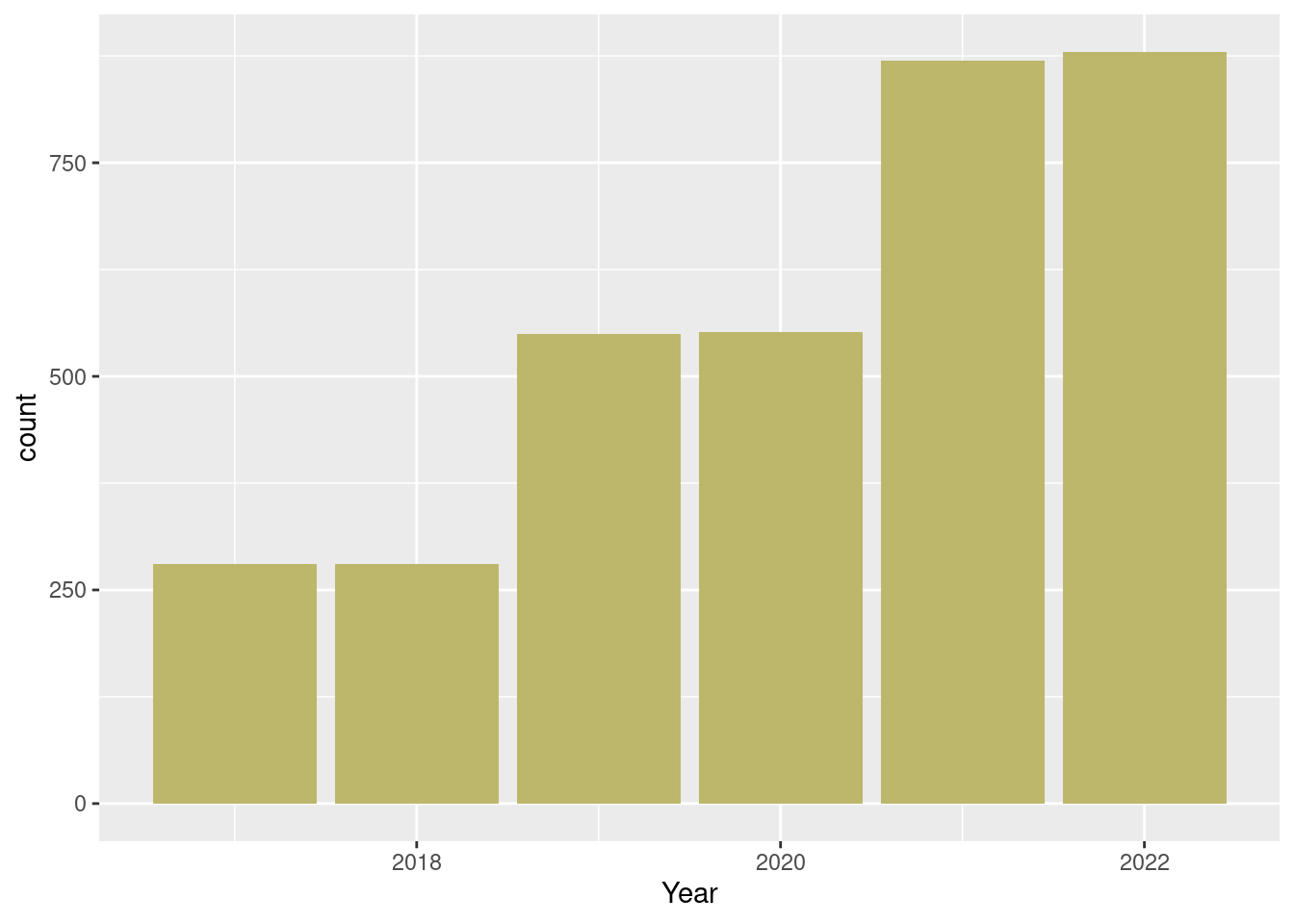
The distribution across years looks much better now.
dat_season |>
  ggplot() +
  geom_bar(aes(
    x = year),
    fill = "darkkhaki") +
  labs(x = "Year") +
  facet_wrap(.~Treatment)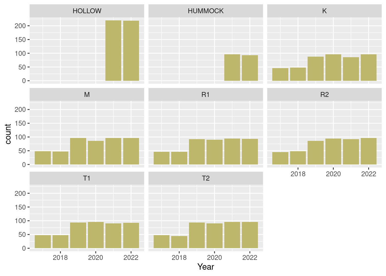
The Edge treatment is now all gone.
dat_season |>
  pivot_longer(
    cols = starts_with("species"),
    values_to = "Species"
    ) |>
  filter(!is.na(Species),
         Species != "NA",
         Species != "dead") |>
  count(Species) |>
  arrange(n) |>
  mutate(Species = fct_inorder(Species)) |>
  ggplot() +
  geom_col(aes(x = Species, y = n),
           fill = "darkkhaki") +
  coord_flip()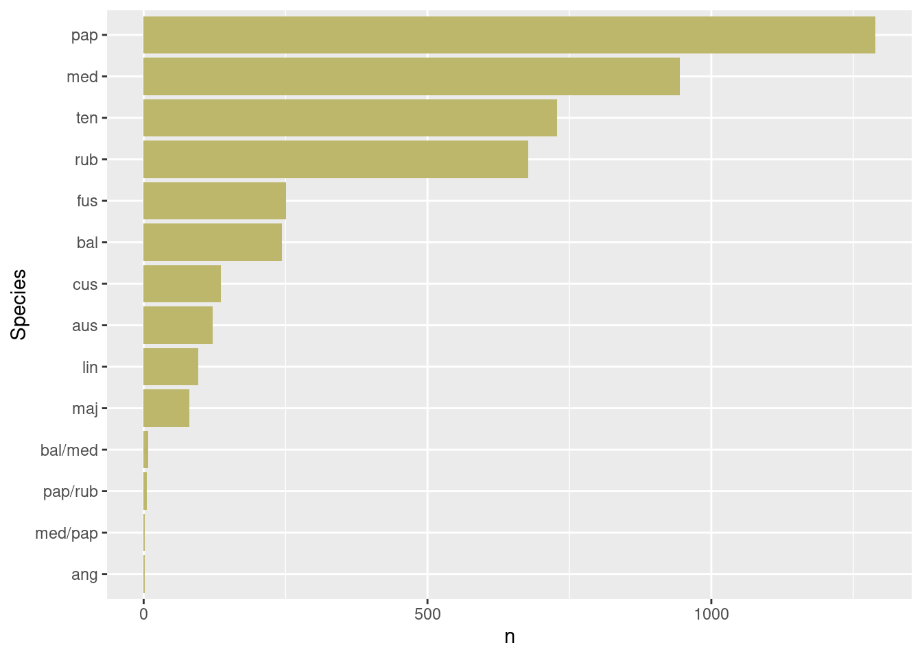
Shagnum papilosum, S. medium, S. tennuis and S. rubellum are the four most common species in the dataset.
dat_season |>
  group_by(year, Treatment) |>
  count() |>
  pivot_wider(names_from = Treatment, values_from = n) |>
  kbl() |>
kable_paper()| year | K | M | R1 | R2 | T1 | T2 | HOLLOW | HUMMOCK |
|---|---|---|---|---|---|---|---|---|
| 2017 | 46 | 48 | 46 | 45 | 47 | 48 | ||
| 2018 | 48 | 47 | 46 | 48 | 47 | 44 | ||
| 2019 | 88 | 96 | 92 | 86 | 94 | 94 | ||
| 2020 | 96 | 86 | 90 | 94 | 96 | 90 | ||
| 2021 | 86 | 96 | 94 | 92 | 90 | 96 | 220 | 96 |
| 2022 | 96 | 96 | 93 | 96 | 92 | 96 | 218 | 93 |
The distribution of data points across treatments now looks much better as well.